To snake or not to snake in the planar Swift–Hohenberg equation
Snaking and nonsnaking scenarios
We study stationary spatially-localised patterns of the cubic-quintic
Swift–Hohenberg equation
$$
u_t = - (1+\Delta)^2 u - \mu u + \nu u^3 - u^5.
$$
This equation describes pattern-forming systems near instabilities with nontrivial
finite spatial wavelengths, and it is widely used to explain the formation and
growth of localised structures.
We pose the Swift–Hohenberg equation on an infinitely-long cylindrical domain
\((x,y) \in S^1 \times \mathbb{R}\), where \(S^1 = \mathbb{R}/2L_x\mathbb{Z}\) for
some real positive number \(L_x\). The patterns that we want to capture are localised
in the \(y\)-direction, and they can be either periodic in \(x\) (of period \(2L_x\)) or
else localised in \(x\) (upon choosing \(L_x \gg 1\)).
We reformulate the stationary Swift–Hohenberg equation as a
spatial-dynamical system, a first-order system in the unbounded
direction \(y\),
$$
U_y = \mathcal{F}(U; \mu, \nu), \qquad U = (u, u_y, u_{yy}, u_{yyy})^t.
$$
The spatial-dynamical formulation is reversible with respect to the reverser
$$
\mathcal{R} \colon (U_1,U_2,U_3,U_4)^t \mapsto (U_1,-U_2,-U_3,-U_4)^t
$$
which corresponds to the reflection symmetry \(y \mapsto -y\) of the stationary
Swift–Hohenberg equation. Localised structures are then interpreted as
homoclinic cycles of the spatial-dynamical system. From this moment onwards, \(\mu\)
will be considered our primary bifurcation parameter, whereas \(\nu\) will be fixed
(unless otherwise stated).
We distinguish between two scenarios for the bifurcation structure of localised
patterns:
-
Nonsnaking scenario: heteroclinic cycles between two
reversible equilibria of the spatial-dynamical system lead to a branch of
symmetric homoclinic orbits. The homoclinic orbits are parametrised by their
width $L$ and exist for parameters \(\mu = \mu(L)\) with \(\mu(L) \to \mu_M\) as
\(L \to \infty\) (Maxwell point). The corresponding bifurcation diagram
features a vertical asymptote.
-
Snaking scenario: heteroclinic cycles between an
equilibrium and a reversible periodic orbit of the spatial-dynamical system
lead to branches of symmetric homoclinic orbits that oscillate between two
distinct parameter values. As we move up on these branches, the localised
structures widen by acquiring additional periodic rolls at an infinite number of
successive saddle-node bifurcations. In general, we expect to find intertwined
snaking branches (corresponding to different symmetries of the
Swift–Hohenberg equation) connected by symmetry-breaking ladders.
Localized rolls: nonsnaking
We fix \(\nu=2\) and continue localised rolls in the parameter \(\nu\). The bifurcation
diagram in the left panel features the squared \(L^2\)-norm of the solutions, which
is a good indicator of the width \(L\) of the computed patterns. When the rolls
are oriented in the \(y\)-direction, their bifurcation diagram resembles the
nonsaking scenario described above. The right panel shows the associated
spatial-dynamics interpretation: the roll pattern corresponds to an equilibrium of
the \(y\)-dynamics.
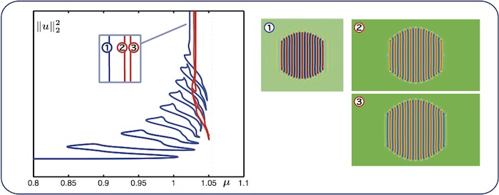
Localized rolls: snaking
If we repeat the computation with rolls oriented in the \(x\)-direction, we find a
snaking bifurcation diagram. In the spatial-dynamics interpretation, the roll
pattern corresponds to a periodic orbit in the \(y\)-dynamics.
Almost-planar localised rolls
Some patterns display both snaking and nonsnaking behaviour in the same bifurcation
diagram. Our starting point is the pattern in the left panel. For decreasing \(\mu\),
we pattern does not snake (panel 2). For increasing \(\mu\), we find a snaking
branch (panel 3). The family of solution profiles along the entire bifurcation
curve can be viewed in the accompanying movie.
Almost-planar localised rolls: nonsnaking
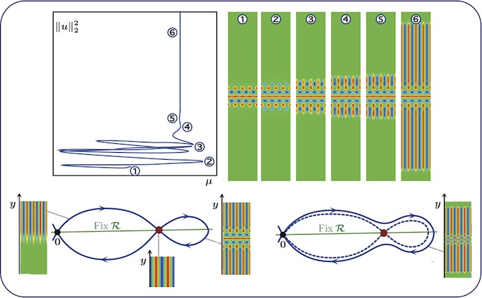
Patterns along the nonsnaking branch can be interpreted in terms of spatial
dynamics: the almost-planar stripe pattern shown in the bottom-right panel
corresponds to a homoclinic orbit that bifurcates from the heteroclinic network
shown in the bottom-left panel. The heteroclinic network involves only equilibria of the
spatial-dynamical system, therefore we are in the nonsaking case.
Almost-planar localised rolls: snaking
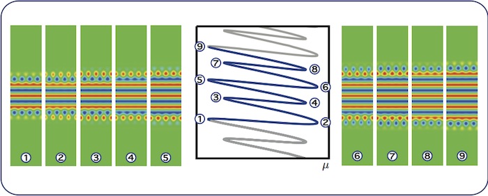
As we move along the snaking branch, the patterns grow horizontal stripes via a
sequence of nine saddle-node bifurcations as shown in panels 1–9. The
spatial-dynamical interpretation (not shown here) involves periodic orbits in the
\(y\)-dynamics, therefore we are in the snaking case.
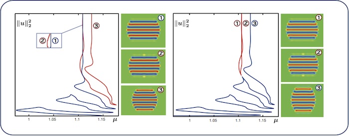
Almost-planar localised rolls: intertwined branches
We find two intertwined snaking branches of almost-planar stripes: the solid branch
corresponds to patterms with symmetry \(u(x,y) = u(x,-y)\), whereas the dashed branch
corresponds to solutions such that \(u(x,y) = - u(L_x-x, -y)\).
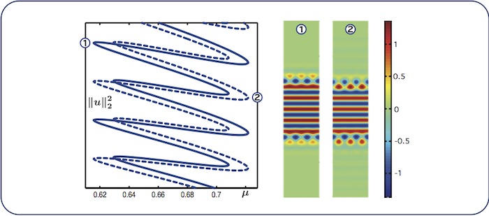
Almost-planar localised rolls: self-connecting branches
We expect to find self-connecting and cross-connecting ladders between
intertwined snaking branches. We show here self-connecing branches that begin and
end at the branch of patterns with symmetry \(u(x,y) = u(x,-y)\).
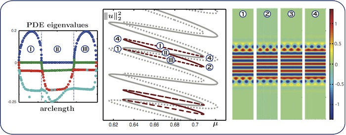
The four rightmost PDE eigenvalues of the states along the ladder
branches are shown in the left panel. The linear stability is computed with
respect to perturbations satisfying Neumann boundary conditions at \(x=0\) and \(x =
L_x\): solutions are stable along the middle part of each ladder.
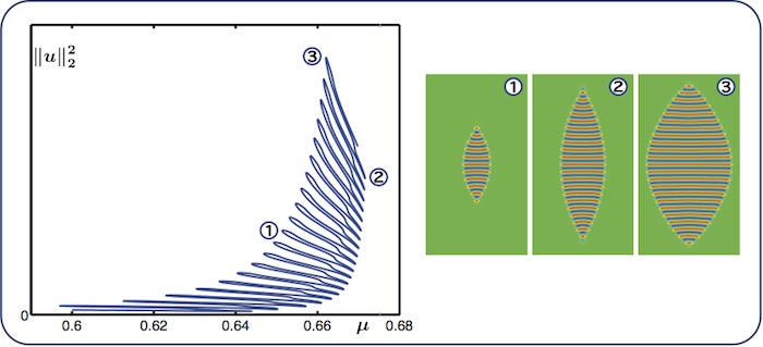
Fully-localised stripes patterns (worms)
We also investigate the bifurcation structure of fully-localised stripes patterns
(known as worms). Spatial dynamics is less effective in this case, as
there is more than one direction in which the patterns may grow. However, we can
still use numerical continuation to explore their parameter dependence.
Worms bifurcate from a branch of radial spots and begin to snake (blue branch),
but eventually the bifurcation diagram approaches a single vertical asymptote.
There also exists a nonsnaking branch (in red) which starts and ends at infinite
\(L^2\)-norm (we can interpret this branch as an isola). The diagrams are obtained
for \(\nu = 2.50081\).
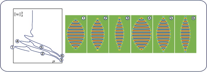
Worms: colliding branches
We repeat similar computations for \(\nu=2.655\) (left) and \(\nu=2.652\) (right). The
blue snaking branch and the leftmost branch of the red isola in the left
panel collide and rearrange themselves upon decreasing \(\nu\), leading to the red
isola and the blue snaking branch shown in the right panel. As a result, the
emerging blue branch in the right panel snakes for longer.
Worms: long snake
As we continue to decrease \(\nu\), more and more nonsnaking branches collide with
the snaking curve, leading to a branch with a very long snaking regime. The
diagram above was obtained for \(\nu = 2\).
Worms: curvature change
In the proximity of the vertical asymptote, the worms change curvature: the sign of
the curvature near the peaked top and bottom ends of the worm patches changes along
the snaking branch. This can also be observed in this animation.
| Author Institutional Affiliation | Department of Mathematics, University of Surrey, UK |
| Author Email | |
| Author Postal Mail | Room 36BC02 / Department of Mathematics / University of Surrey / Guildford, Surrey / GU2 7XH / United Kingdom / Tel: +44 (0)1483 68 3615 |
| Notes | Based on a paper published in SIADS, Vol. 9, No. 3, pp. 704-733 |
| Keywords | Swift-Hohenberg, planar patterns, snaking, localized structures |