1. Motivation

It is common knowledge that the same substance can exist in different forms or phases and that, depending on temperature and pressure, two or more phases of the same substance can coexist at thermodynamical equilibrium.

In the case of alloys or mineral compounds one can observe regions occupied by two different crystalline phases separated by an interface or there may be singular points, i.e., junctions, where three or more equally preferred phases meet (see Figure 1).

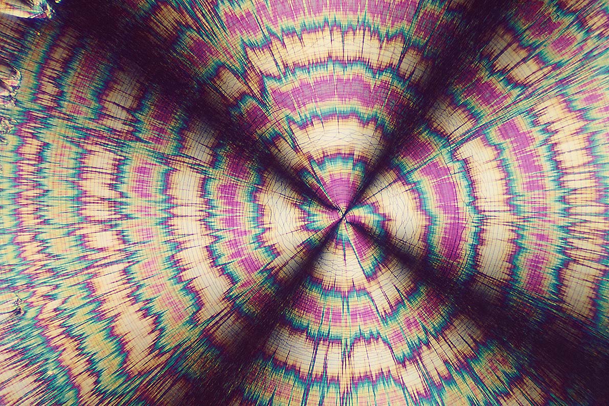
Figure 1. Hippuric acid (David Malin): a junction point. The junction point lays at the intersection of two reflection lines that correspond to the interfaces between four regions.

Another interesting structure is observed when polyhedral regions with different phases tile space with an almost regular pattern. Examples of such situations observed experimentally are presented in Figures 2 and 3.

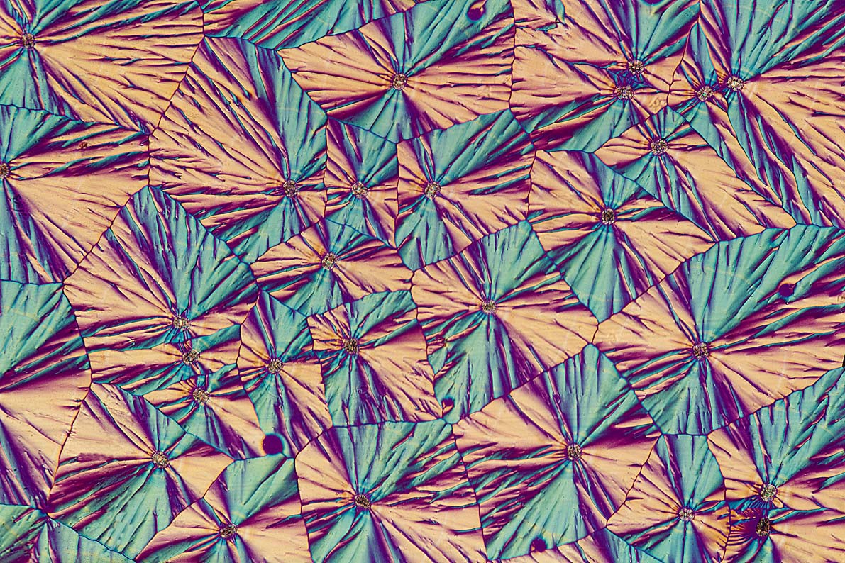
Figure 2. Tiling, Vitamin C crystals (David Malin). Tiling of the plane with structured multiphase cells. Note the junction point in each cell.

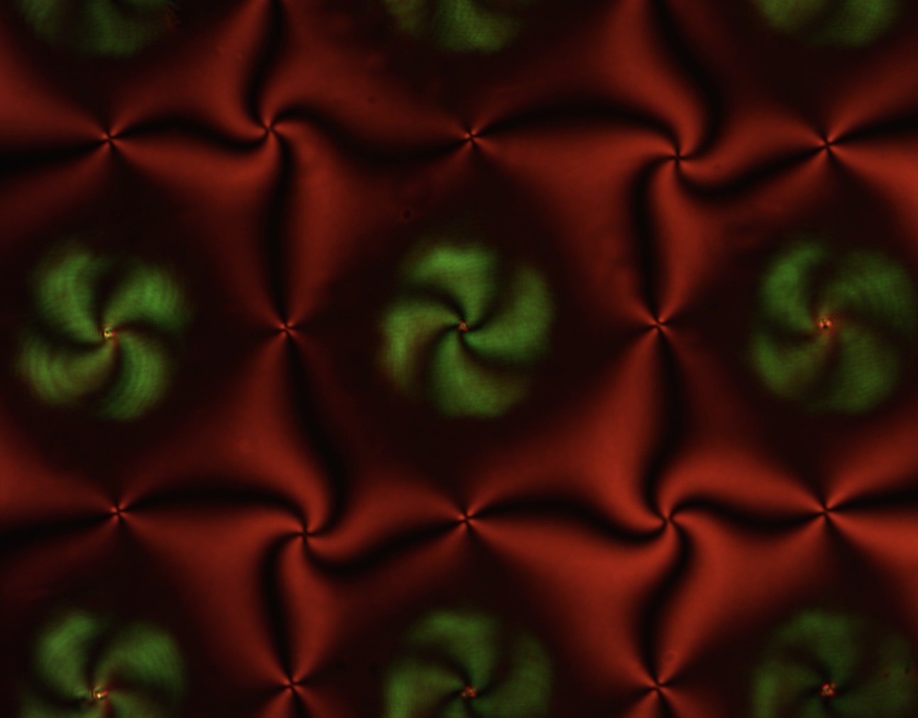
Figure 3. Square lattice structure of a liquid crystal illuminated by periodic laser lights.

The aim of our paper [3] is to discuss a simple mathematical model that can describe an amazing variety of multiphase states that include multiple junctions and tilings. A nonnegative function \(W:\mathbb{R}^m\rightarrow\ \mathbb{R}^+\), \(m>1\), with a finite number of zeros is used to model the bulk free energy density of a material that, at thermodynamical equilibrium, can exist in several equally preferred phases corresponding to the zeros \(a_1,\ldots,a_N\in\mathbb{R}^m\) of \(W\). In some cases the vector \(u\) describes the mass fraction of each element but the number of minimal energy phases, \(N\), may or may not equal \(m\). Sometimes the different phases are different orientations of a crystal or different crystalline structures of the same elements at roughly the same concentrations.

Under the simplifying assumption that the interfacial energy density can be modeled by the isotropic quantity \(\frac{\epsilon^2}{2}\vert\nabla u\vert^2\), where \(0<\epsilon\ll 1\) is a parameter that measures the importance of interfacial versus bulk energy, the free energy of the material contained in a bounded region \(\Omega\subset\mathbb{R}^n\), \(n\geq 1,\) can be modeled by the Allen-Cahn functional:

(1.1)

\(J_\Omega(u)=\int_\Omega\big(\frac{\epsilon^2}{2}\vert\nabla u\vert^2+W(u)\Big) dx,\)

where the map \(\Omega\ni x\rightarrow u(x)\in\mathbb{R}^m\) describes the distribution of an order parameter \(u(x)\in\mathbb{R}^m\) in \(\Omega\): \(u(x)\approx a_j\) means that at \(x\in\Omega\) the material is approximately in phase \(a_j\) and \(u(x)\in\mathbb{R}^m\setminus\{a_1,\ldots,a_N\}\) means that at \(x\) it is in some mixed or disordered state. To model the tendency of the system to evolve toward states of minimal energy we can consider the gradient system associated with \(J_\Omega\). This depends on the choice of the Hilbert space \(H\) that gives the metric with respect to which we compute the gradient of \(J_\Omega\). For \(H=L^2(\Omega;\mathbb{R}^m)\) and writing \(W_u(u)\,\,\text{for}\,\,(\frac{\partial W(u)}{\partial u_1},\ldots,\frac{\partial W(u)}{\partial u_m})^\top\) we obtain the parabolic Allen-Cahn system of equations

(1.2)

\(\left\{\begin{array}{l} u_t=\epsilon^2\Delta u-W_u(u),\;\;x\in\Omega,\;\;\\ \frac{\partial u}{\partial\nu}=0,\;\;x\in\partial\Omega,\\ u(0,x)=u_0. \end{array}\right.\)

This system of nonlinear partial differential equations is probably the simplest model for phase separation phenomena. Given an initial state \(u_0\), for small \(\epsilon>0\), we can distinguish different behaviors in the dynamics of (1.2). In an initial time interval of order \(\mathrm{O}(1)\) the evolution is essentially dictated by the ODE \(u_t=-W_u(u)\) that, depending on the structure of \(u_0\), evolves the solution \(u^\epsilon(t,x,u_0)\) towards the set of minima of \(W\), and as a result \(\Omega\) is partitioned into subregions where \(u^\epsilon\) is approximately constant and equal to one of the \(a_j\). That is, the space is divided in subregions occupied by different coexisting phases of the material. These subregions are separated by an interface of thickness \(\mathrm{O}(\epsilon)\) across which \(u^\epsilon\) makes a transition from a neighborhood of one of the minima of \(W\) to a neighborhood of another. Following this first period, the so called separation stage, \(u^\epsilon\) develops high gradients across the interfaces and the two terms on the right hand side of (1.2) become comparable throughout \(\Omega\), and a second, slower, evolution of the material structure begins during which \(u^\epsilon\) keeps its partitioned structure while the phase boundaries evolve with speed of order \(\mathrm{O}(\epsilon^2)\). This evolution stage often leads to a reduction of the measure and the disappearance of one or more connected components of the subregion corresponding to one of the phases. This phenomenon is called coarsening and involves changes in the topological structure of the interface. In any case, the asymptotic fate of the evolution is a solution \(u:\Omega\rightarrow\mathbb{R}^m\) of the stationary vector Allen-Cahn equation \[\epsilon^2\Delta u=W_u(u)\quad \text{for}\quad x\in \Omega,\] \[\frac{\partial u}{\partial n} = 0 \quad \text{on} \quad \partial\Omega,\] which is the Euler-Lagrange equation of the functional (1.1).

We are interested in the local structure of the phase-junction points where three or more subregions corresponding to different phases meet. Therefore, we focus on one of these points that we assume to coincide with the origin \(0\in\mathbb{R}^n\) and dilate the space around \(0\) via the transformation \(x\rightarrow \epsilon x\). This, in the limit \(\epsilon\rightarrow 0\), leads to the study of entire solutions \(u:\mathbb{R}^n\rightarrow\mathbb{R}^m\) of the rescaled equation

(1.3)

\(\Delta u=W_u(u),\;\;x\in\mathbb{R}^n,\)

which is formally the Euler-Lagrange equation of the functional

(1.4)

\(J(u)=\int_{\mathbb{R}^n}\Big(\frac{1}{2}\vert\nabla{u}\vert+W(u)\Big)dx.\)

Entire solutions of (1.3) are also relevant to model the tiling of space observed in physical experiments.

The study of general entire solutions of (1.3) is very hard. The main difficulty is that, if \(W\) has two or more zeros, \(J_\Omega\) is not convex and there is no a priori method for characterizing the regions where \(u(x)\) is near to one or another of the \(a_1,\ldots,a_N\). We restrict to symmetric potentials \(W\) and to symmetric solutions. The restriction to the symmetric setting has both physical and mathematical motivations. From the physical point of view we observe that symmetry is ubiquitous in nature. Symmetric structures are observed at the junction of three or four coexisting phases in physical space. Similar structures appear at the singularities of soap films and compounds of soap bubbles. We also note that in the modeling of crystalline phase transitions of alloys it is quite natural to assume that \(W\) enjoys some kind of symmetry that reflects the symmetry of the underlining microscopic crystal lattice of the alloy. In such situations \(W\) can be assumed to depend on a vector order parameter \(u\in\mathbb{R}^m\) which describes the fraction of the components of the alloy in each of \(m\) sublattices of the microscopic crystal lattice, and \(u=a_j\), \(j=1,\ldots,N\), corresponds to a pure phase [4]. To give the idea consider the planar lattice shown in Figure 4. Assume that the lattice is composed of three sublattices: white, blue and red. In this situation the potential \(W\) is a function of the atomic fractions \(u_1,u_2\) and \(u_3\) of the white, blue and red sublattices. If the atomic interaction is the same independently of the color of the atoms, then \(W\) satisfies \[\begin{split} & W(u_1,u_2,u_3)=W(u_2,u_3,u_1)=W(u_3,u_1,u_2),\\ & W(u_1,u_2,u_3)=W(u_1,u_3,u_2). \end{split}\] Therefore \(W\) is invariant under the symmetry group of the equilateral triangle with vertices in \((1,0,0)\), \((0,1,0)\) and \((0,0,1)\) that may coincide with the zeros \(a_1,a_2,a_3\) of \(W\).

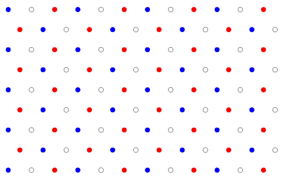
Figure 4. The symmetry of the underlyining microscopic lattice which is consistent with \(W\) having the symmetry of a triangle with minima at the red, white, and blue states.

2. The main theorems

In [3] we present a systematic study of symmetric bounded entire solutions of (1.3). We assume that \(W\) is invariant under a finite reflection group \(\Gamma\) acting on \(\mathbb{R}^m\) and that there is a reflection group \(G\) acting on the domain space \(\mathbb{R}^n\). Since we intend to include also periodic patterns we consider both the cases where \(G\) is a finite or an infinite (discrete) reflection group.

We assume that \(G\) and \(\Gamma\) are related by a homomorphism \(f:G\rightarrow\Gamma\) and define a map \(u:\mathbb{R}^n\rightarrow\mathbb{R}^m\) to be \(f\)-equivariant if

(2.1)

\(u(gx)=f(g)u(x),\;\;\text{ for }\;g\in G,\;x\in\mathbb{R}^n.\)

This notion of equivariance with respect to a homomorphism describes all symmetric patterns. Let us give some basic examples when \(n=m=1\).

(1) Take \(G=\Gamma=\{I,\sigma\}\), with \(I:\mathbb{R}\rightarrow\mathbb{R}\) the identity map, \(\sigma:\mathbb{R}\rightarrow\mathbb{R}\) the antipodal map \(\sigma(x)=-x\), and let \(f:G\rightarrow G\) be the identity. Then (2.1) takes the form \[u(\sigma(x))=\sigma(u(x))\quad\Leftrightarrow\quad u(-x)=-u(x),\] and a map \(u:\mathbb{R}\rightarrow\mathbb{R}\) is \(f\)-equivariant if and only if it is odd.

(2) With \(G=\Gamma=\{I,\sigma\}\) as in (1), let \(f\) be the trivial homomorphism that maps \(\sigma\) into \(I\). In this case (2.1) reads \[u(\sigma(x))=u(x)\quad\Leftrightarrow\quad u(-x)=u(x)\] and a map \(u\) is \(f\)-equivariant if and only if it is even.

(3) Next, we consider the discrete reflection group \(G\) of \(\mathbb{R}\) generated by \(s_0=\sigma\) and by the reflection \(s_1(x)=2-x\). The elements of \(G\) are the reflections \(s_k(x)=2k -x\) and the translations \(t_k(x)=x+2k\) (\(k\in\mathbb{Z}\)). We take \(\Gamma=\{I,\sigma\}\) as before, and define \(f\) such that \(f(s_k)=\sigma=s_0\), \(f(t_k)=I\). In this case (2.1) takes the form \[\begin{split} &u(s_k(x))=s_0(u(x))\quad\Leftrightarrow\quad u(2k-x)=-u(x),\;\;k\in\mathbb{Z},\\ &u(t_k(x))=I(u(x))\quad\Leftrightarrow\quad u(2k+x)=u(x),\;\;k\in\mathbb{Z}. \end{split}\] The function \(u(x)=\sin (\pi x)\) which satisfies these conditions, is an example of \(f\)-equivariant map, and the same is true for any odd \(2\)-periodic map.

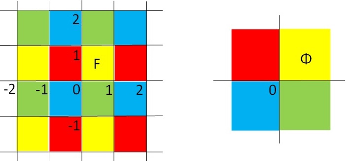
Figure 5. On the left: a square lattice generated by the reflections along the lines \(x_2=k\) and \(x_1=l\) (\(k,l\in \mathbb{Z}\)) parallel to the coordinate axes. On the right: the dihedral group \(D_2\) generated by the two reflections along the coordinate axes.

Similarly, when \(n=m=2\) the finite reflection groups of the plane are the dihedral groups \(D_k\) (\(k\geq 1\)), which are the symmetry groups of regular polygons. A basic example of a discrete reflection group of the plane is the group \(G\) generated by the reflections along the lines \(x_2=k\) and \(x_1=l\) (\(k,l\in \mathbb{Z}\)) cf. Figure 5 (left). If we take \(G=\Gamma=D_2\) (cf. Figure 5 (right)), and \(f\) to be the identity, then a \(f\)-equivariant map \(u=(u_1,u_2):\mathbb{R}^2\to\mathbb{R}^2\) satisfies the conditions: \[u_1(-x_1,x_2)=-u_1(x_1,x_2),\;\; u_2(-x_1,x_2)=u_2(x_1,x_2) \text{ for }\; x=(x_1,x_2)\in\mathbb{R}^2,\] \[u_1(x_1,-x_2)=u_1(x_1,x_2),\;\; u_2(x_1,-x_2)=-u_2(x_1,x_2) \text{ for }\; x=(x_1,x_2)\in\mathbb{R}^2.\] In particular, a point belonging to the \(x_i\) (\(i=1,2\)) coordinate axis is mapped on the \(u_i\) coordinate axis, and \(u(0,0)=(0,0)\).

The reflection hyperplanes of a finite or discrete reflection group partition the space into identical cells that are called fundamental domains. For instance, the square \(F=(0,1)\times (0,1)\) is a fundamental domain of the discrete reflection group depicted in Figure 5 (left), while a sector of angle \(\pi/k\) is a fundamental domain of the dihedral group \(D_k\) (cf. Figure 5 (right) when \(k=2\)). In the one dimensional example (1) above, the half-line \(F=(0,\infty)\) is a fundamental domain of \(G=\Gamma=\{I,\sigma\}\). Finally, in example (3) above, the interval \(F=(0,1)\) is a fundamental domain of the corresponding discrete reflection group \(G\).

We characterize the homomorphisms which allow for the existence of \(f\)-equivariant maps that send a fundamental domain \(f\) for the action of \(G\) on \(\mathbb{R}^n\) into a fundamental domain \(\Phi\) for the action of \(\Gamma\) on \(\mathbb{R}^m\):

(2.2)

\(u(\overline{F})\subset\overline{\Phi}.\)

In the case of the one dimensional example (1) above, condition (2.2) means that \(u(x)\geq 0\), \(\forall x\in \overline F=[0,\infty)\). Similarly, in the case of example (3) above, condition (2.2) means that \(u(x)\geq 0\), \(\forall x\in \overline F=[0,1]\). By analogy with the scalar case \(m=1\), and for the coherence of the terminology, we refer to these homomorphisms and to the maps that satisfy (2.2) as positive.

If, as in [3], we assume that \(W\) is invariant under \(\Gamma\) and that \(W\) has a unique zero, say \(a_1\), in \(\overline{\Phi}\), from (2.2) it follows that, for \(x\in\overline F\), \(u(x)\) remains at a distance from all the zeros of \(W\) different from \(a_1\). This is of central importance in the proofs of Theorems 2.1 and 2.2 below. Not all homomorphisms allow for the existence of nontrivial \(f\)-equivariant maps that satisfy (2.2). To see that positive homomorphisms need to satisfy a particular condition observe that, if \(u\) is an \(f\)-equivariant satisfying (2.2), and \(x\in\overline{F}\) belongs to \(P\), one of the hyperplanes that bound \(f\), we have \[u(x)=u(s(x))=f(s)u(x)\in\overline{\Phi},\] where \(s\in G\) is the reflection in \(P\). It follows that \(u(x)\in\overline{\Phi}\) is a fixed point of \(f(s)\) and therefore, since \(u(x)\) in the interior of \(\Phi\) implies \(\gamma u(x)\neq u(x)\) for any \(\gamma\in\Gamma\setminus\{I_m\}\), we necessarily have that \(u(x)\) belongs to one of the hyperplanes that bound \(\overline{\Phi}\). The conclusion is that \(f(s)\) is either one of the reflections associated to the hyperplanes that bound \(\overline{\Phi}\) or the product of some of these reflections. Therefore we define

Definition 1. Let \(f\) be a fundamental domain of \(G\), bounded by the hyperplanes \(P_1, \ldots ,P_l\), correponding to the reflections \(s_1, \ldots, s_l\). We say that a homomorphism \(f: G \to \Gamma\) is positive if there exists a fundamental domain \(\Phi\) of \(\Gamma\), bounded by the hyperplanes \(\Pi_1,\ldots, \Pi_k\), such that for every \(i=1, \ldots,l\), there is \(1\leq k_i\leq k\) and \(\tilde{\Pi}_1,\ldots,\tilde{\Pi}_{k_i}\in\{\Pi_1,\ldots, \Pi_k\}\) such that

(2.3)

\(\ker(f(s_i)-I_m)=\cap_{j=1}^{k_i}\tilde{\Pi}_j.\)

That is, the set of points fixed by the orthogonal map \(f(s_i)\) is one of the hyperplanes \(\Pi_j\), or the intersection of several of them.

Positive homomorphisms have certain mapping properties that relate the reflections associated to the walls of a fundamental domain \(f\) to the reflections associated to the walls of a corresponding region \(\Phi\). These properties are instrumental to show that minimizing in the class of \(f\)-equivariant maps that satisfy (2.2) does not affect the Euler-Lagrange equation and renders a smooth solution of (1.3). The proof of this fact is based on a quite sophisticated use of the maximum principle for parabolic equations. We prove that, provided \(f\) is a positive homomorphism, the \(L^2\) gradient flow associated to the functional (1.4) preserves the positivity condition (2.2). By a careful choice of certain scalar projections of the vector parabolic equation that describes the above mentioned gradient flow, we show that this fact is indeed a consequence of the maximum principle.

Based on this we prove two abstract existence results: Theorem 2.1 which concerns the case where \(G\) is a finite reflection group and Theorem 2 that treats the case of a discrete (infinite) group \(G\).

Theorem 2.1 (Point group, \(u:\mathbb{R}^n\to\mathbb{R}^m\)). Under the hypotheses that

• \(W\) is invariant with respect to a reflection point group \(\Gamma\), and that the closure of the fundamental domain \(\overline \Phi\) contains a unique zero of \(W\), say \(a_1\),
• there exist: a finite reflection group \(G\) acting on \(\mathbb{R}^n\), and a positive homomorphism \(f : G \to \Gamma\) (cf. Definition 1) that associates \(\Phi\) with the fundamental domain \(f\) of \(G\),

there exists an \(f\)-equivariant solution \(u\) of (1.3), \(u(gx)=f(g) u(x)\), for \(g \in G\), which is positive, and connects the phases at infinity:

 

(2.4)

\(u(\overline F) \subset \overline \Phi \text{ (positivity)},\)

(2.5)

\(|u(x)-a_1|\leq Ce^{-cd(x,\partial D_1)}, \ x \in D_1,\)

where \(D_1= \mathrm{Int}\left( {\cup_{g\in f^{-1}(\mathrm{Stab(a_1)})} g \overline{F}} \right)\).

In the case where a discrete reflection group acts on the domain space, we give a slightly different version of the theorem. Since the fundamental region of a discrete reflection group is bounded or has a cylindrical structure, the exponential estimate applies when the corresponding lattice blows up. By rescaling, this is equivalent to multiplying the gradient of the potential in (1.3) by a factor \(R^2\), and consider the lattice in the domain space as fixed.

Theorem 2.2 (Lattice). Under the hypotheses that

• \(W\) is invariant with respect to a reflection point group \(\Gamma\), and that the closure of the fundamental domain \(\overline \Phi\) contains a unique zero of \(W\), say \(a_1\),
• there exist: a discrete reflection group \(G\) acting on \(\mathbb{R}^n\), and a positive homomorphism \(f : G \to \Gamma\) (cf. Definition 1) that associates \(\Phi\) with the fundamental domain \(f\) of \(G\),

there exists an \(R_0\) such that for all \(R>R_0\), there exists an \(f\)-equivariant solution \(u_R:\mathbb{R}^n\to\mathbb{R}^m\) (\(u_R(gx)=f(g) u_R(x)\), for \(g \in G\)) to system

(2.6)

\(\Delta u_R - R^2 W_u(u_R) = 0, \text{ for } x\in \mathbb{R}^n,\)

which is positive, and connects the phases:

(2.7)

\(u(\overline F) \subset \overline \Phi \text{ (positivity)},\)

(2.8)

\(|u_R(x)-a_1|\leq Ce^{-cRd(x,\partial D_1)}, \ x \in D_1,\)

where \(D_1= \mathrm{Int}\left( {\cup_{g\in f^{-1}(\mathrm{Stab(a_1)})} g \overline{F}} \right)\).

From (2.2) and the \(f\)-equivariance of \(u\) it follows that

(2.9)

\(u(g\overline{F})\subset f(g)\overline{\Phi},\;\text{ for }\;g\in G.\)

For instance, going back to the situation described in Figure 5, let \(G\) be the discrete reflection group depicted in Figure 5 (left), and let \(\Gamma=D_2\) as in Figure 5 (right). We consider the positive homomorphism \(f:G\to\Gamma\) such that the reflection along \(u_i=0\) (\(i=1,2\)) in the range, is the image by \(f\) of the reflections along \(x_i=k\) (\(k\in\mathbb{Z}\)) in the domain. By taking \(F=(0,1)\times (0,1)\) (cf. the yellow square in Figure 5 (left)), and \(\Phi=(0,\infty)\times (0,\infty)\) (cf. the yellow quadrant in Figure 5 (right)), we deduce from (2.2) and the \(f\)-equivariance of \(u\), that any square in the domain is mapped into a quadrant with the same colour (cf. Figure 5). Moreover, since we can show that the map \(u\) only vanishes on \(\mathbb{Z}\times\mathbb{Z}\), we obtain according to Figure 5, the configuration of the vortices of \(u\): at the points \((k,l)\in\mathbb{Z}\times\mathbb{Z}\) where both \(k\) and \(l\) are either even or odd, \(u\) has a vortex of degree \(+1\), while at the remaining points \((k,l)\in\mathbb{Z}\times\mathbb{Z}\), \(u\) has a vortex of degree \(-1\). In this way, we can model the experiment presented in Figure 3, where a liquid crystal is illuminated by laser lights centered at the points \(2\mathbb{Z}\times 2\mathbb{Z}\). We point out that in this context the vector parameter \(u\) is related to the orientation of the molecules. For the general theory of light-matter interacion in liquid crystals we refer to [6].

Therefore, besides its importance for the proofs of Theorems 2.1 and 2.2, the mapping property (2.2) is a source of information on the geometric structure of the vector valued map \(u\). The fact that (2.9) holds true in general in the abstract setting of the present analysis can perhaps be regarded as one of the significant results in [3]. From the mathematical point of view, symmetry plays an essential role in the derivation of pointwise estimate for solutions of (1.3). Indeed by exploiting the symmetry we show, as in [1] and [2], the existence of minimizers of \(J_\Omega\) that map fundamental domains in the domain \(x\)-space into fundamental domains in the target \(u\)-space. A basic consequence of this is the existence of minimizers that in certain sub-domains avoid all the minima of \(W\) but one. It follows that in each such sub-domain the potential \(W\) can be considered to have a unique global minimum. This is a key point since, as we have observed, for potentials with two or more global minima, it is very difficult to determine a priori in which subregions a minimizer \(u\) of \(J_\Omega\) is near to one or another of the minima of \(W\) (cf. [7], [8]).

Due to the variety of choices for \(n\) and \(m\) (the dimensions of domain and target space), the reflection groups \(G\) and \(\Gamma\), and the homomorphism \(f:G\rightarrow\Gamma\), we will deduce from Theorems 2.1 and 2.2 the existence of various complex multi-phase solutions of (1.3) including several types of lattice solutions. With the help of the pictures below we will briefly describe these constructions detailed in [3].

Our first example is the triple junction, a solution of (1.3) that corresponds to the situation where three different phases meet at a junction point. In this case we take \(n=m=2\), \(G=\Gamma=D_3\) the symmetry group of the equilateral triangle and \(f:D_3\rightarrow D_3\) the identity. Figure 6 (right) shows the partition of \(\mathbb{R}^2\) in fundamental domains under the action of \(D_3\). We assume that the only zero of \(W:\mathbb{R}^2\rightarrow\mathbb{R}\) in \(\overline{\Phi}\) is \(a_1=(1,0)\). Then the invariance of \(W\) under \(D_3\) implies that the zeros of \(W\) are \(a_1\), \(a_2=(-1/2,\sqrt{3}/2)\) and \(a_3=(-1/2,-\sqrt{3}/2)\), the vertices of an equilateral triangle with center \(O\). The stabilizer of \(a_1\), the subgroup of \(\Gamma=D_3\) that leaves \(a_1\) fixed, is \(\mathrm{Stab}(a_1)=\{I_2,\sigma_1\}\) with \(\sigma_1\) the reflection in the line \(u_2=0\). This and \(f=I\) imply that \(D_1=\{x\in\mathbb{R}^2: x_1>0, \vert x_2\vert<\sqrt{3} x_1\}\) and Theorem 2.1 yields a solution \(\mathbb{R}^2\ni x\rightarrow u(x)\in\mathbb{R}^2\) of (1.3) that in \(D_1\) converges exponentially to \(a_1\) as the distance \(d(x,\partial D_1)\) diverges to \(+\infty\). If we interpret Figure 6 (right) as the partition of the domain space \(\mathbb{R}^2\) under the action of \(G=\mathbb{R}^2\), \(D_1\) corresponds to the union of the yellow and the green sectors. The existence of the triple junction solution of (1.3) was first established in [5].

Similarly, for \(n=m=3\), Theorem 2.1 implies the existence of a quadruple junction, a solution \(u:\mathbb{R}^3\rightarrow\mathbb{R}^3\) of (1.3) that corresponds to the situation where four different phases meet at a junction point. To see this take \(G=\Gamma=\mathcal{T}\), the symmetry group of the tetrahedron \(A_1,A_2,A_3,A_4\) in Figure 6 (left) and \(f=I\). The fundamental domains for the action of \(\mathcal{T}\) on \(\mathbb{R}^3\) are the \(24\) cones with vertex in \(O\) generated by the \(24\) triangles on the boundary of the cube depicted in Figure 6 (left). If we assume that \(a_1=A_1\), then the invariance of \(W\) under \(\Gamma=\mathcal{T}\) implies that \(W\) has exactly four zeros that coincide with \(A_1,A_2,A_3,A_4\). Since \(f=I\) we can identify domain and target space and think of the cones in Figure 6 (left) as the partition of \(\mathbb{R}^3\) both in domain and target space. Then \(D_1\) corresponds to the union of the six cones that have \(A_1\) on their boundary and \(\mathbb{R}^3\) is decomposed in four cones congruent with \(D_1\), one for each of the \(A_i\) and in each of these four cones we have exponential convergence of the solution \(u\) to the corresponding \(A_i\). We mention that the existence of the quadruple junction solution of (1.3) was first established in [9].

Actually the abstract character of Theorem 2.1 allows to extend the above results to general \(n=m\geq 3\) to show the existence of a \(n+1\)-junction, a solution \(u:\mathbb{R}^n\rightarrow\mathbb{R}^n\) of (1.3) that model the situation where \(n+1\) phases meet at a point. In this general setting \(G=\Gamma=\mathcal{T}_n\), with \(\mathcal{T}_n\) the symmetry group of the hypertetrahedron with \(n+1\) vertices. \(W\) has \(n+1\) zeros that coincide with the vertices of the hypertetrahedron. Now \(\mathbb{R}^n\) is divided in \(n+1\) congruent cones one for each of the zeros of \(W\) and in each of such cones \(u\) converges exponentially to the corresponding zero of \(W\).

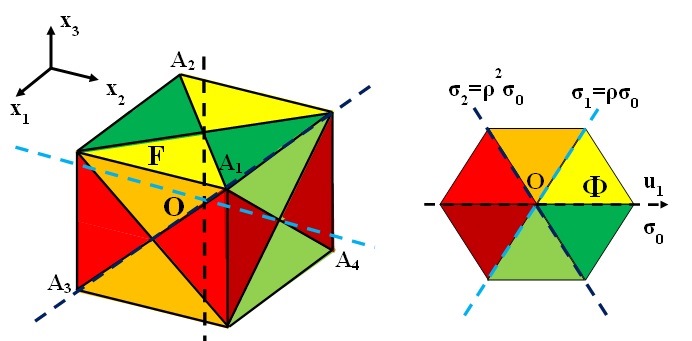
Figure 6. Fundamental domains for the action of \(\mathcal{T}\) on \(\mathbb{R}^3\) (left) and for the action of \(D_3\) on \(\mathbb{R}^2\) (right). The \(f\)-equivariant solution \(u:\mathbb{R}^3\rightarrow\mathbb{R}^2\) of (1.3) given by Theorem 2.1 maps fundamental domains into fundamental domains with the same color. In particular \(u\) maps the infinite double cone (union of four fundamental domains) generated by \(O\) and by the two yellow triangles into the sector \(\Phi\).

Beside the above examples Theorem 2.1 can describe junction points with quite complex structure. We give an example where the dimension of the range (\(m=2\)) is intrinsically distinct from the dimension of the domain (\(n=3\)). Indeed we take \(G=\mathcal{T}\) acting on \(\mathbb{R}^3\) and \(\Gamma=D_3\) acting on \(\mathbb{R}^2\) cf. Figure 6.

With \(s_0\) and \(s_1\) the reflections in the plane \(OA_1A_2\) and \(OA_3A_4\) respectively and \(s_2\) the reflection in the plane \(OA_1A_4\), we consider the positive homomorphism \(f:\mathcal{T}\rightarrow D_3\) defined by \[\begin{split} &f(s_0)=f(s_1)=\sigma_0,\quad\text{the reflection in the line}\:\:u_1=0,\\ &f(s_2)=\sigma_1,\quad\text{the reflection in the line}\:\:u_2=\sqrt{3}u_1. \end{split}\] If \(W\) has six zeros, one in the interior of each of the fundamental domains for the action of \(D_3\) on \(\mathbb{R}^2\), the positive \(f\)-equivariant solution \(u:\mathbb{R}^3\rightarrow\mathbb{R}^2\) of (1.3) given by Theorem 2.1 maps fundamental domains into fundamental domains with the same color. In particular, the four fundamental domains determined by the two yellow triangles and by their symmetric with respect to \(O\) are mapped into \(\overline{\Phi}\) and correspond to \(D_1\). \(\mathbb{R}^3\) is divided in six cones congruent with \(D_1\) and in each of these cones \(u\) converges exponentially to the corresponding zero of \(W\). To give an idea of the vector field \(\mathbb{R}^3\ni x\rightarrow u(x)\in\mathbb{R}^2\) identify the plane \((u_1,u_2)\) with the plane through \(O\in\mathbb{R}^3\) orthogonal to \(OA_1\) and assume that the axis \(u_2=0\) is parallel to \(A_3A_4\). Then \[\begin{split} & x\;\text{in the plane}\;\;OA_3A_4\quad\Rightarrow\quad u(x)\;\;\text{parallel to}\;A_3A_4,\\ & x\;\text{in the plane}\;\;OA_1A_2\quad\Rightarrow\quad u(x)\;\;\text{parallel to}\;A_3A_4,\\ & x\;\text{in the plane}\;\;OA_1A_4\quad\Rightarrow\quad u(x)\;\;\text{orthogonal to}\;OA_1A_4. \end{split}\]

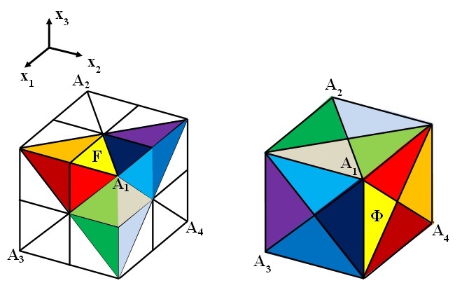
Figure 7. Fundamental domains for the action on \(\mathbb{R}^3\) of \(\mathcal{K}\) (left) and \(\mathcal{T}\) (right). The \(f\)-equivariant solution \(u:\mathbb{R}^3\rightarrow\mathbb{R}^3\) of (1.3) given by Theorem 2.1 maps fundamental domains into fundamental domains with the same color.

In the next example, the symmetry group \(\mathcal{K}\) of the cube acts on the domain \(\mathbb{R}^3\), while the symmetry group \(\mathcal{T}\) of the tetrahedron acts in the target space \(\mathbb{R}^3\) (cf. Figure 7). We can identify the vertices of the tetrahedron with the vertices \(A_1,A_2,A_3,A_4\) of the cube. Then each symmetry plane of the tetrahedron is also a symmetry plane of the cube. Let \(s_1\) the reflection in the plane \(OA_1A_2\), \(s_2\) the reflection in the plane \(OA_1A_4\), \(s_3\) the reflection in the plane \(\{x_2=0\}\), and \(s_5\) the reflection in the plane \(OA_2A_3\). Then the homomorphism \(f:\mathcal{K}\rightarrow\mathcal{T}\) defined by the conditions

(2.10)

\(f(s_1)=s_1,\;f(s_2)=s_2,\;f(s_3)=s_5\)

is a positive homomorphism and any positive \(f\)-equivariant map maps fundamental domains into fundamental domains with the same color as indicated in Figure 7.

If \(W\) has \(24\) zeros, one in the interior of each fundamental domain, the set \(D_1\) is the double cone generated by the yellow triangle and the center of the cube in Figure 7 and \(\mathbb{R}^3\) is partitioned in \(24\) cones congruent with \(D_1\) and in each of these cones the solution \(u\) given by Theorem 2.1 converges exponentially to the corresponding zero of \(W\) and \(u\) is a model for a \(24\)-junction point.

If instead the potential \(W\) has for instance only four zeros (located at the vertices of the tetrahedron \(A_1\),\(A_2\),\(A_3\) and \(A_4\)), then \(D_1\) is the union of two octants symmetric with respect to the center of the cube and the domain space \(\mathbb{R}^3\) is partitioned in four congruent cones as indicated in Figure 8.

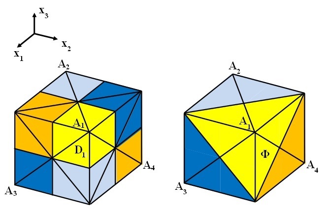
Figure 8. The partition of the domain space \(\mathbb{R}^3\) when \(W\) has four minima on the vertices of the tetrahedron. In this case \(D_1=\{x\in\mathbb{R}^3: x_ix_j>0,\;1\leq i,j\leq 3\}\) and the solution \(u\) of (1.3) given by Theorem 2.1 satisfies: \(u(x)\rightarrow A_1\), for \(\min_i\vert x_i\vert\rightarrow+\infty,\;x\in D_1\).

Next we use Theorem 2.2 to give examples of solutions of (1.3) with a periodic character which model the situation where regions with different phases tile the space and repeat itself with an almost regular pattern. In Figure 5 we have already considered an example of this kind. The solution \(u:\mathbb{R}^2\rightarrow\mathbb{R}^2\) considered in Figure 5 is periodic of period \(2\) in both variables and therefore the pattern in Figure 5 can be generated by applying the translations \[t_{hk}x=(x_1+2h,x_2+2k),\;\;(h,k)\in\mathbb{Z}\times\mathbb{Z} \] to the elementary cell: the union of the four squares that touch the origin \(O\).

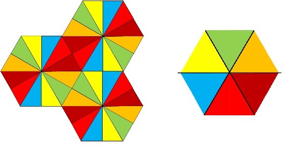
Figure 9. Fundamental domains for the actions on \(\mathbb{R}^2\) of \(G^\prime\) (left) and \(D_3\) (right). The \(f\)-equivariant solution \(u_R\) of (1.3) given by Theorem 2.2 maps fundamental domains into fundamental domains with the same color.

In Figure 9 we present a more involved example of lattice solution than the square lattice described in Figure 5 above. In the domain \(\mathbb{R}^2\) we consider the discrete reflection group \(G\) generated by the reflection \(s_0\) in the line \(x_2=0\), the reflection \(s_1\) in the line \(x_2=x_1/\sqrt{3}\) and the reflection \(s_2\) in the line \(x_2=-\sqrt{3}(x_1-1)\). In the target space \(\mathbb{R}^2\) we take \(\Gamma=D_3\). In Figure 9 (left) we show the partition of \(\mathbb{R}^2\) in fundamental domain under the action of \(G\).

The subgroup generated by \(s_0\) and \(s_1\) coincides with \(D_6\), the symmetry group of the regular hexagon, and with the stabilizer of the origin (the subgroup of the \(g\in G\) that leaves \(O\) fixed). The discrete reflection group \(G\) contains also the translation group \(T\) generated by the translations \[t_\pm(x)=x+\big(\frac{3}{2},\pm\frac{\sqrt{3}}{2}\big).\] The positive homomorphism \(f:G\rightarrow D_3\) is defined by

\[\begin{split} & f(s_0)=\;\;\text{the reflection in the line}\;u_2=0,\\ & f(s_1)=\;\;\text{the reflection in the line}\;u_2=-\sqrt{3}u_1,\\ & f(s_2)=\;\;\text{the reflection in the line}\;u_2=-\sqrt{3}u_1. \end{split}\]

Figure 9 describes the mapping properties of an \(f\)-equivariant positive solution \(u_R\) of (1.3) given by Theorem 2.2. In this case the elementary cell is the hexagon union of the \(12\) triangles with a vertex at the origin. As hinted in Figure 9, under the action of the translation group \(T\), the elementary cell tiles the whole plane. If we assume that \(a_1\) is in the interior of \(\Phi\) and therefore that \(W\) has exactly six zeros, one in each of the fundamental domains for the action of \(D_3\) on \(\mathbb{R}^2\), then the set \(D_1\) is the union of all yellow triangles in the plane. The solution \(u\) depends on \(R>0\) and (2.8) in Theorem 2.2 implies

\[\lim_{R\rightarrow+\infty}u_R(x)=a_1,\;\;x\in D_1.\]

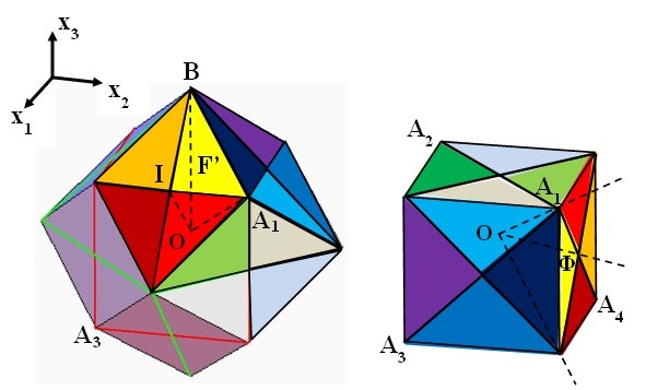
Figure 10. Fundamental domains for the action on \(\mathbb{R}^3\) of \(\mathcal{K'}\) (left) and \(\mathcal{T}\) (right). The fundamental domain \(F'\) of \(\mathcal{K'}\) is a pyramid with basis the triangle \(A_1BI\) and vertex in \(O\). Under the action of the point group \(\mathcal{K}\), \(F'\) generates the rhombic dodecahedron \(C\) (left) which tiles the domain space \(\mathbb{R}^3\) when translated by the elements of \(T\). The \(f\)-equivariant solution \(u_R:\mathbb{R}^3\rightarrow\mathbb{R}^3\) of (1.3) given by Theorem 2.2 maps fundamental domains into fundamental domains with the same color. Note in particular that \(u\) maps \(\cup_{t\in T}(\overline{F^\prime}\cup-\overline{F^\prime})\) into \(\overline{\Phi}\).

Our last example is a solution \(u:\mathbb{R}^3\rightarrow\mathbb{R}^3\) of (1.3) that corresponds to a tiling of the three dimensional space (cf. Figure 10). For this example \(n=m=3\), \(\Gamma=\mathcal{T}\) the symmetry group of the tetrahedron and \(G\) is the discrete reflection group \(\mathcal{K'}\) acting in \(\mathbb{R}^3\) which is generated by the reflections \(s_1\), \(s_2\), \(s_3\) and \(s_4\) in the planes \(P_1:=OA_1A_2\), \(P_2:=OA_1A_4\), \(P_3:=\{x_2=0 \}\) and \(P_4:=\{x_1+ x_3=2 \}\). These planes bound the fundamental domain \(F'\) of \(\mathcal{K'}\) with vertices at the points \(O\), \(A_1\), \(I:=(1,0,1)\) and \(B:=(0,0,2)\) (cf. Figure 10). In this case, the positive homomorphism \(f\) is defined by (2.10) and by

\[f(s_4)=s_5.\]

The homomorphism \(f\) associates \(F'\) to the fundamental domain \(\Phi\) of \(\mathcal{T}\) bounded by the planes \(OA_1A_2\), \(OA_1A_4\) and \(OA_2A_3\). The point group of \(\mathcal{K'}\), that is the stabilizer of the origin, is the group \(\mathcal{K}\), the symmetry group of the cube and we have \(\mathcal{K'}=\{tk: k\in\mathcal{K},\; t\in T\}\), where \(T\) is the translation group of \(\mathcal{K'}\). \(T\) is generated by the translations with respect to the vectors \(t_1:=(2,0,2)\), \(t_2:=(0,2,2)\) and \(t_3:=(0,-2,2)\).  The elementary cell \(C=\cup_{g \in \mathcal{K}} \overline{gF'}\) is a rhombic dodecahedron (the union of the \(48\) fundamental domains that touch the origin cf. Figure 10) that tiles the three dimensional space when translated by the elements of \(T\) (space filling tessellation with rhombic dodecahedra is the crystal structure in which often are found garnets and other minerals like pyrite and magnetite). Several structures are possible for the solution \(u_R\) given by Theorem 2.2 depending on the position of \(a_1\in\overline{\Phi}\). For instance if \(a_1\) is in the interior of \(\Phi\), \(W\) has \(24\) zeros and \(D_1=\cup_{t\in T}(F^\prime\cup-F^\prime)\) and the space is partitioned in \(24\) sets congruent with \(D_1\) and, in each of these sets, \(u_R(x)\) converges to corresponding zero of \(W\) as \(R\rightarrow+\infty\).

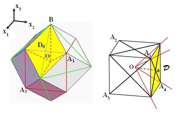
Figure 11. If \(a_1=(0,1,0)\), \(W\) has six minima (one in the middle of each side of the tetrahedron). In this case the positive \(f\)-equivariant solution \(u_R:\mathbb{R}^3\rightarrow\mathbb{R}^3\) given by Theorem 2.2 satisfies \(\lim_{R\rightarrow+\infty}u_R(x)=(0,1,0)\) for \(x\in D_1=\cup_{t\in T}(D_0\cup-D_0)\), \(D_0\) the pyramid with basis the rhombus defined by the points \(A_1,B,(1,-1,1),(2,0,0)\), and vertex in \(O\).

If instead \(a=(0,1,0)\) \(W\) has six zeros the middle points of the sides of the tetrahedron (cf. Figure 11). \(D_1=\cup_{t\in T}(D_0\cup-D_0)\) with \(D_0\) the pyramid with basis the rhombus defined by the points \(A_1,B,(1,-1,1),(2,0,0)\), and vertex in \(O\). Theorem 2.2 implies

\[\lim_{R\rightarrow+\infty}u_R(x)=(0,1,0),\;x\in D_1.\]

Funding: PWB was supported in part by NSF DMS-0908348, DMS-1413060, and the IMA. GF was partially supported by the IMA. PS was partially supported by and Fondo Basal AFB170001 CMM-Chile and Fondecyt postdoctoral grant 3160055.

References

[1]   N. D. Alikakos and G. Fusco, Entire solutions to equivariant elliptic systems with variational structure, Arch. Rat. Mech. Anal. 202, No. 2 (2011), pp. 567-–597.

[2]   N. D. Alikakos and P. Smyrnelis, Existence of lattice solutions to semilinear elliptic systems with periodic potential, Electron. J. Diff. Equ., 15 (2012), pp. 1--15.

[3]   P. Bates, G. Fusco, and P. Smyrnelis, Multiphase solutions to the vector Allen-Cahn equation: crystalline and other complex symmetric structures. Entire solutions with six-fold junctions to elliptic gradient systems with triangle symmetry, Archive for Rational Mechanics and Analysis 225, No. 2 (2017), pp. 685-–715.

[4]   R. J. Braun, J. W. Cahn, G. B. MacFadden, and A. A. Wheeler, Anisotropy of interfaces in an ordered alloy: a multiple-order-parameter model, Trans. Roy. Soc. London, A, 355 (1997), pp. 1787--1833.

[5]   L. Bronsard, C. Gui, and M. Schatzman, A three-layered minimizer in \(\mathbb{R}^2\) for a variational problem with a symmetric three-well potential, Comm. Pure. Appl. Math. 49, No. 7 (1996), pp. 677--715.

[6]   M. G. Clerc, M. Kowalczyk, and P. Smyrnelis, Symmetry breaking and restoration in the Ginzburg-Landau model of nematic liquid crystals, Journal of Nonlinear Science 28, No. 3 (2018), pp. 1079--1107.

[7]   G. Fusco, Equivariant entire solutions to the elliptic system \(\Delta u=W_u(u)\) for general \(G\)-invariant potentials, Calc. Var. Part. Diff. Eqs. 49, No. 3 (2014), pp. 963--985.

[8]   G. Fusco, On some elementary properties of vector minimizers of the Allen-Cahn energy, Comm. Pure Appl. Analysis 13, No. 3 (2014), pp. 1045--1060.

[9]   C. Gui and M. Schatzman, Symmetric quadruple phase transitions, Ind. Univ. Math. J. 57, No. 2 (2008), pp. 781--836.