This article presents work that was completed by a number of contributors including Balázs Bárány, Erik Boczko, Nathan Breitsch, Xue Gong, Richard Buckalew, Bastien Fernandez, Tomas Gedeon, Luke Morgan, Gregory Moses, and Alexander Neiman. This project received support from NIH-NIGMS grant R01GM090207.

Background: Yeast Autonomous Oscillations

We have been studying ensemble models of the mitotic cell division cycle in which cells in one fixed region of the cycle \(S\) (Signaling) produce chemical signals that affect the growth and development rate of cells in another fixed region \(R\) (Responsive).

Our motivation has been to understand Yeast Autonomous Oscillations (YAO), a phenomenon that has been observed in experiments for at least 60 years [8,15] and remains a topic of interest for various biological reasons [9,22,5]. In YMO, budding yeast (Saccharomyces cerevisiae) enter stable periodic oscillations between aerobic and anaerobic modes of metabolism. In Figure 1 we present an example of a culture entering YMO with a period of about 4 hours.

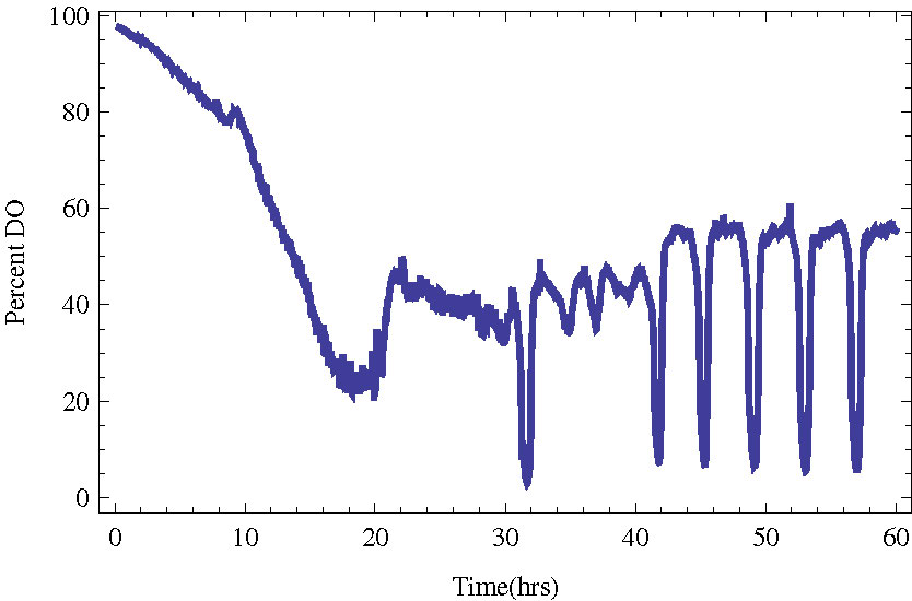
Figure 1. Budding yeast in a bioreactor entering stable metabolic oscillations (YMO). The measured quantity is the dissolved oxygen in the bioreactor.

A link between YAO and the cell division cycle (CDC) was noticed as early as [15,25], but this connection was obscured by the fact that the YAO oscillations had a shorter period than the CDC in the experiments. The connection seems to have been ignored until it was again noted in genetic expression time series [13,14].

Since yeast is a model organism, it is important to understand the interconnectedness of its CDC and metabolism. Yeast are used in many bio-engineering processes and understanding their metabolism and cell cycle is of interest in these applications. Further, the CDC is a topic of intense general interest and progress has been made in identifying many genetic and biochemical agents controlling the CDC.

The CDC of budding yeast consists of 4 distinct phases:

• G1: growth phase, begins with cell division;
• S: replication phase, begins with budding;
• G2: second growth phase;
• M: narrowing or 'necking', ends in cell division.

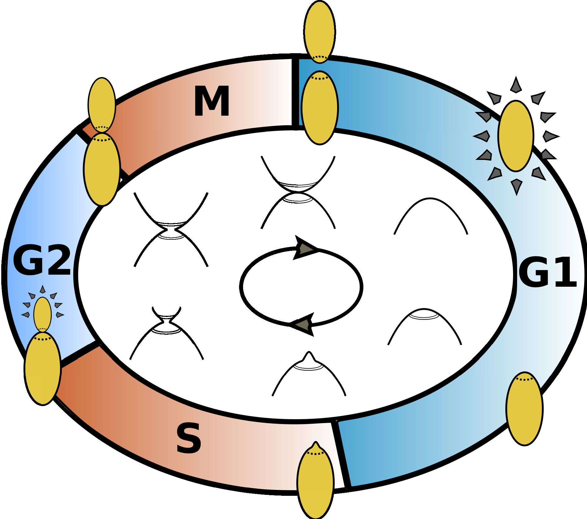
Figure 2. Illustration of the cell cycle of budding yeast.

In [2], based on data in [18], we proposed cell cycle clustering as a possible explanation of the interaction between YAO and the CDC. By clustering we mean groups of cells traversing the CDC in near temporal synchrony, i.e., a type of phase-synchronization. It does not involve spatial clustering, since YAO occur in well-mixed bioreactors. In [2,26] we studied general forms of (1) (below) with the hypothesis that cells in one part of the CDC may influence CDC progression of cells in other parts of the CDC through diffusible metabolites or other chemicals. For example, a cohort of cells in the critical replication phase might effect metabolism production and the metabolites may in turn inhibit cell growth in the later part of the G1 phase, thus setting up a feedback mechanism in which YAO and CDC clustering are intertwined.

Model, Simulations, and Experiments

The model we introduce below is based on two well-established biological facts about the cell cycle:

B1. Different and complex chemistry occurs in each phase.
B2. Chemicals in the media can influence cells differently in different phases.

See [16] for a review of some of the biological literature supporting these two facts in the context of budding yeast.

Guided by B1 and B2 we began studying a model of the cell cycle as a circle and on this circle we consider a collection of \(n\) cells; the position of the \(i\)-th cell is denoted by \(x_i \in [0,1) \equiv S^1\). Cells in a specific region \(S \subset [0,1)\) (Signaling) affect the development rate of cells in another fixed region \(R \subset [0,1)\) (Responsive), see Figure 3. The progression of the cells is governed by the equations:

\(\frac{dx_i}{dt} = \begin{cases} 1, \quad \textrm{if} \quad x_i \notin R, \\ 1+ f(I) , \quad \textrm{if} \quad x_i \in R, \end{cases} \qquad 1 \le i \le n,\)

(1)

where

\(I(\bar{x}) \equiv \frac{\#\{j:x_j \in S\}}{n} \quad \) (fraction of cells in the signaling region).

(2)

The "response function" \(f(I)\) in (1) should satisfy \(f(0) = 0\), \(f(I) > -1\), and be monotone, but may be non-linear, for instance sigmoidal, and either positive or negative. When a cell reaches \(1\) (division) it returns to \(0\) (birth).

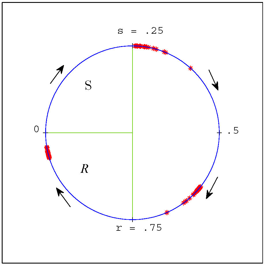
Figure 3. Our coordinate representation of the cell cycle and (weakly clustered) groups of cells from a negative feedback simulation with \(n = 200\) and parameter values \(s=.25\) and \(r = .75\). Positions of individual cells are denoted by red asterisks. Stochastic noise was added in this simulation to separate cells and illustrate robustness. In this coordinate system the \(S\) region is the interval \([0,.25)\) and the \(R\) region is \([.75,1)\).

The behaviour of a cell in this model is simple: It progresses through the cycle with a normalized rate of 1, unless it is in the responsive region \(R\) and there are simultaneously cells in the signaling region \(S\) influencing its rate of progress.

By a cluster, we mean a group of cells that are synchronized in the CDC. If a cluster is stable in an ideal model, then in a real system with noise we expect to observe weakly synchronized groups of cells. We found in numerical experiments using variations of the model and random initial conditions that solutions tend to form clusters very frequently. See Figure 3 for an example of a clustered final distribution from a simulation.

Guided by these simulations and some preliminary analysis of the model, we sought to verify the existence of CDC clusters in experiments. We found clustering in two types of oscillating yeast cultures using both bud index and cell density data [2,24]. See Figure 4.

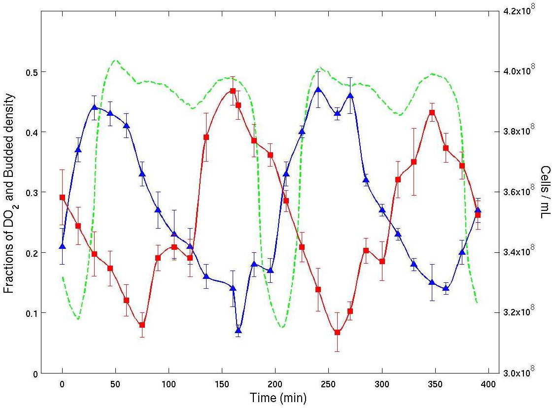
Figure 4. Experimental time series from a continuous culture of budding yeast in YMO. Dissolved \(O_2\) % (green), bud index % (blue) and cell density (red) are plotted vs. time. The average cell cycle period was about 400 minutes. The plot shows clearly that the bud index (% of cells with buds from microscopy) and cell density (by flow cytometry) are both entrained with the oscillation in dissolved \(O_2\). The plot shows that there are two temporal clusters of cells of nearly the same number of cells. They are traversing the CDC in anti-phase.

Mathematical questions

While the discovery of clusters in yeast experiments was very satisfying, we are primarily Mathematicians and we were confronted by many questions about the dynamics of (1). For example,

1. When do clustered solutions exist?
2. What are the differences between systems that Synchronize and those that Cluster?
3. What determines how many clusters form?
4. When are clusters asymptotically stable?

We have sought to answer these questions in subsequent years. It turns out that the dynamics of the model are very rich and contain many surprises. We describe some of our results in the rest of this article, beginning with the first question.

In the model (1), if a cluster of cells is synchronized, then that cluster will persist, so we may reduce the dimension of the system to \(k\), the number of clusters. Among all clustered states, it is natural to first consider those that are are associated with periodic solutions.

Definition 1. A clustered solution \(\{ x_i(t) \}_{i=1}^k\) is \(k\) cyclic if \(\exists\) a time \(d>0\) s.t.:

\[\begin{split} x_i(d) &=x_{i+1}(0) \quad \forall \quad i=1, \ldots, k-1, \\ & \textrm{and} \quad x_k(d)=x_1(0) \mod 1. \end{split}\]

There are two Special Cases:

• \(k=1\) - synchronized.
• \(k=n\) - uniform.

In the uniform solution cells are "maximally spread out".

It turns out that cyclic solutions always exist.

Theorem 2. If \(k\) is a divisor of \(n\), then a cyclic \(k\) cluster solution exists consisting of \(n/k\) cells in each cluster.

In particular, the synchronized solution always exists (obvious) as does the uniform solution (not obvious).

Poincaré Section, Return Map, and the Map \(F\)

We say that a hyper-surface \(\Sigma\) is a Poincaré section if \(\Sigma\) is transverse to \(\dot{\phi}^t(x)\) at every \(x \in \Sigma\) and every solution reaches \(\Sigma\) in finite time. For any \(x \in \Sigma\), \(\phi^t(x)\) will return to \(\Sigma\) for a minimal \(t^*>0\). Define \(\Pi(x)\) to be the return point.

For our system, since \(\dot{x}_i >0\), any set \(\{x_i = c\}\) is a Poincaré section. We will use \(\Sigma = \{x_1 = 0\}\). A fixed point of \(\Pi\) is a periodic orbit for the flow.

Our strategy will be to use the map \(F\) illustrated in Figure 5. The map \(F\) is defined by flowing until \(x_k(t) =1\), then reordering indices. \(F: S \rightarrow S\), \(S = \{0 \le x_2 \le \ldots \le x_k \le 1 \}\). This definition of \(F\) is a useful tool for the proof of existence of \(k\)-cyclic solutions.

\(F^k\) is the Poincaré return map.

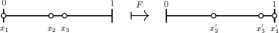
Figure 5. An illustration of the map \(F\) with \(k=3\); \(F(x_1, x_2) = (x'_1, x'_2)\).

Idea of the Proof of Theorem 2:

\(F\) permutes the boundary of \(S\) + Brouwer FPT \(\Rightarrow\)
                  \(F\) has interior fixed point \(\iff\) \(k\)-cyclic solution.

We can also use \(F\) to study solutions for small \(k\) in detail. For example in Figure 6 we present \(F\) calculated explicitly for \(k=2\) in both possible cases. From \(F\) we can infer all dynamics in the 2-cluster submanifold.

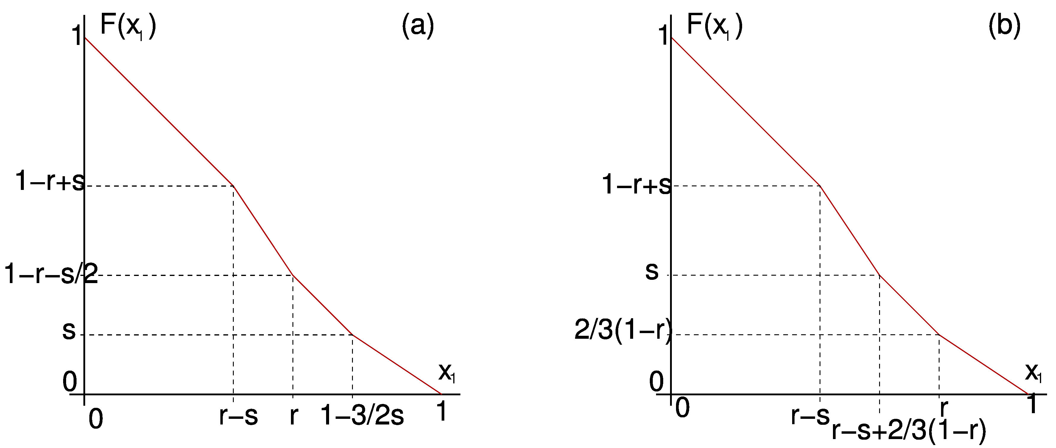
Figure 6. \(F\) for \(k=2\) with positive feedback in the two possible cases: (a) \(r + \frac{3}{2} s < 1\). (b) \(r + \frac{3}{2} s \ge 1\).

Negative vs. Positive Feedback

If the regions \(R\) and \(S\) are small (\(|R|+|S| <1/2\)) then it is not hard to see that clustered solutions may exist in which clusters never interact with each other and that such solutions are neutrally stable.

Let \(M = \lfloor (|R|+|S|)^{-1} \rfloor\). We can show that \(M\) is the maximum number of clusters that can exist without interactions. In Figure 7 we plot the number of clusters that form in simulations compared with \(M\) for both positive and negative feedback.

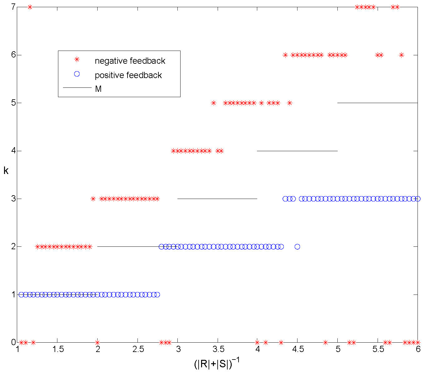
Figure 7. Numerical experiments with positive and negative feedback. The number of clusters formed starting from random initial conditions, compared with \(M\). With positive feedback we only observe synchronized solutions and solutions with \(k \le M\). For negative feedback clusters usually form. The number of clusters \(k\) depends on the size of the regions \(R\) and \(S\) and we always observe \(k>M\).

For positive feedback we can prove the following proposition: The synchronized solution is the only asymptotically stable periodic solution.

For negative feedback, on the other hand: An isolated cluster is unstable under negative feedback.

Stable clustering apparently requires negative feedback and interaction between clusters.

Stability of \(k\)-cyclic solutions for negative feedback

Next we turn our attention to the question of stability of \(k\)-cyclic solutions which happens to be quite fascinating.

Note that our model has two parameters \(s\) and \(r\) that describe the sizes of the signaling and responsive regions \(S\) and \(R\). Our parameter space is thus the triangle \(0 \le s \le r \le 1\). We showed that given \(k\) this parameter triangle is subdivided regularly into \(k^2\) smaller triangles that describe the stability of cyclic solutions [3]. In Figure 8 we produce these regions for the cases \(k = 2, \ldots, 9\). In these plots, Blue indicates Asymptotically Stable, White signifies Neutrally Stable, and Red means Unstable.

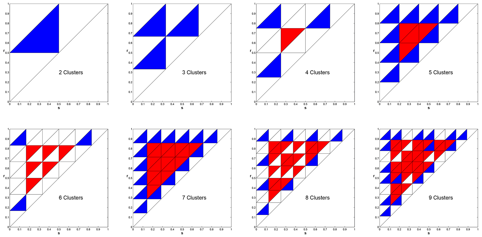
Figure 8. Stability properties of the \(k\)-cyclic solutions in parameter space for \(k=2, \ldots, 9\). Blue - Asymptotically Stable, White - Neutral, Red - Unstable.

Amazingly these stability regions depend on number theoretic relationships. In the case that \(k\) is prime, the coloring of regions is absolutely regular. For \(k\) composite the arrangement of stable and neutral regions is much more complex. As it turns out that if one numbers the regions with a corner on the boundary, starting from any corner, then the triangle numbered \(i\) is stable (blue) if and only if \(i\) and \(k\) are relatively prime [17,21]!

In [3] we made the following conjecture based on the Figure 9 and similar plots.

Conjecture: Clustering is Universal for Negative Feedback. Specifically, the stable regions cover the interior of the parameter triangle \(0 < s < r < 1\).

This conjecture has recently been proven in the case that the feedback function, \(f\), is linear [21]. The proof relies on the number theoretic relationships of the stable triangles. Figure 10 illustrates one of the main ideas of the proof. If \(k\) is composite, and, \((k,i)\) are not relative prime, the corresponding triangle, though not stable is covered by a larger triangle corresponding to \(k / \textrm{gcd}(k,i)\) and \(i / \textrm{gcd}(k,i)\).

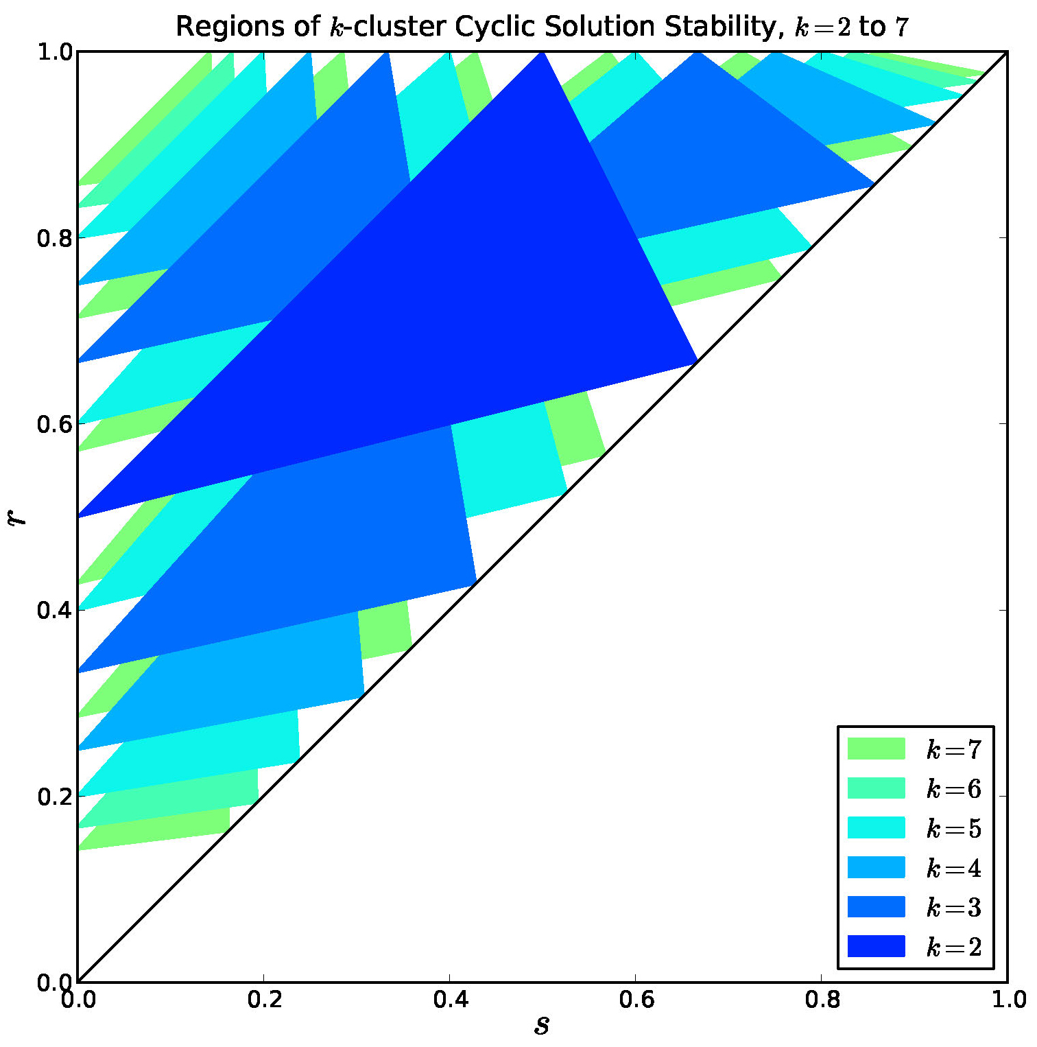
Figure 9. Overlay of stable regions for \(k = 2, \ldots, 7\). Every interior point is covered by a stable region for some \(k\).

Note in Figure 9 that there are many regions of bi-stability or multi-stability.

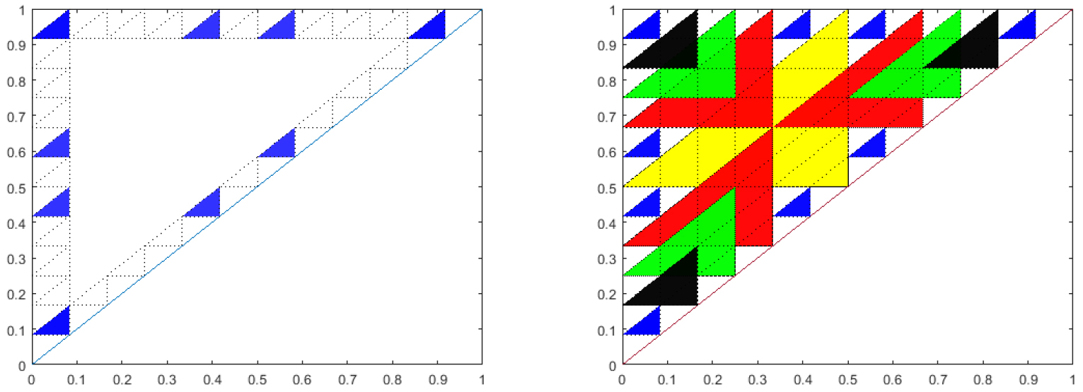
Figure 10. Left: Blue triangles are the relatively prime sub-triangles for \(k=12\). Right: Overlay of the relatively prime sub-triangles for \(k=2\) (yellow), 3 (red), 4 (green), 6 (black) over \(k=12\) (blue).

Positive Feedback and Instability of the Uniform Solution

In Figure 11, we present the same plots, but with positive feedback. For positive feedback clustered solutions are never stable. This was proved in [1]  for any \(k\ge 2\), including the case \(k=n\), i.e., the uniform solutions is unstable under positive feedback.

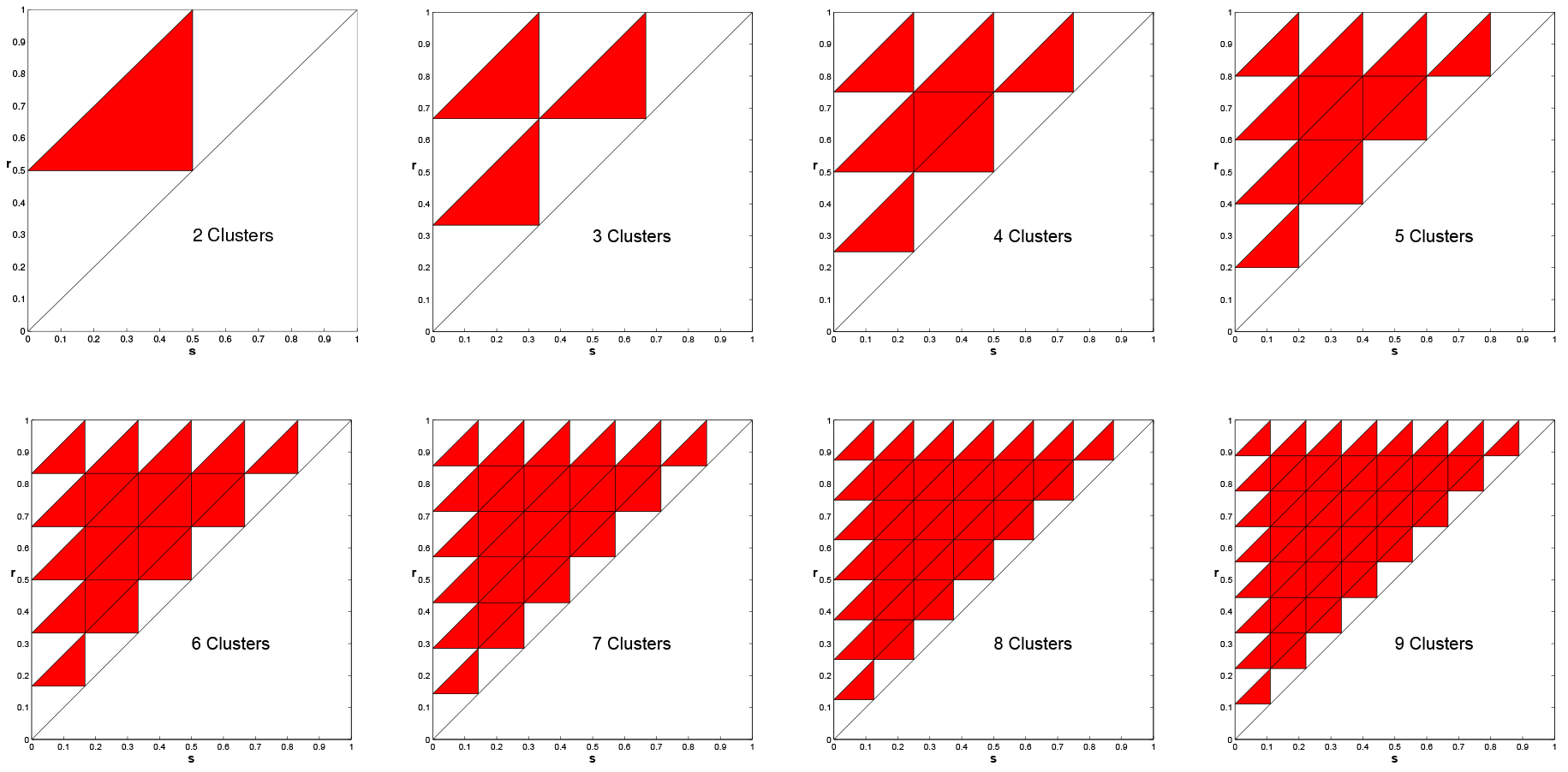
Figure 11. Instability of clustered solutions for positive feedback, \(k = 2, \ldots, 9\). Multiple Clusters are NEVER Asymptotically Stable.

Note that for negative feedback in plots in Figure 8 the interior triangles are mostly red, indicating instability of the \(k\) clustered solution. In [1] we proved instability for over half of the interior subtriangles under negative feedback. Again, this includes the uniform solution (\(k=n\)).

In terms of applications, uniform and cyclic solutions with \(k\) small are very different in kind. In the uniform solution the cells are "maximally spread out"; this corresponds to the "steady-state" solution found in PDE models of the cell cycle. Without feedback, but with some form of dispersion or noise such as random division times, the steady state solution is stable [7,12]. These results suggest that in real systems with a feedback mechanism, there is competition between the phenomena of clustering and dispersion. Dispersion due to internal and external noise sources tends to stabilize the uniform solution, while feedback tends to destabilize the uniform solution and stabilize either synchronous or clustered solutions. Gong et al. [11] used yeast autonomous oscillation data and simulations with biologically relevant noise to conclude that a relatively large feedback, on the order of 30% slow down for negative feedback, was necessary to destabilize the uniform solution and produce coherent clustering as seen in the experiments.

Some Conclusions for General Cell Cycle Feedback

In summary we have obtained some answers to the mathematical questions presented earlier.

• Systems that Synchronize and Cluster are very different!
• Positive Feedback robustly produces Synchronization.
• Clustering is a robust phenomenon for Negative Feedback:

- Number of clusters depends of size of \(S\) and \(R\).
- Not dependent on functional form of feedback.
- It occurs for large open sets of parameter values.
- It requires interaction among clusters.

Some variations on the model

In (1) we ignore variables that represent signaling agents, assuming that the time-scales of the dynamics of these variables are significantly shorter than the time-scale of the CDC. Buckalew [4] considered a model with a term \(z\) representing some substrate factor that influences growth rate and \(z\) itself is coupled with \(\bar{x}\):

\(\dot{x}_i = \begin{cases} 1, \quad \textrm{if} \quad x_i \notin R, \\ 1+ f \left( z \right), \quad \textrm{if} \quad x_i \in R, \end{cases} \qquad \dot{z} = \alpha I - \mu z\).

(3)

Here \(I\) is the fraction of cells in \(S\) as before.

Immediately one sees that some results do not carry over, e.g., an isolated cluster is not linearly unstable under negative feedback, and in fact is linearly stable.

In [4] Buckalew studied how to recover the immediate model from the mediated model and found that the limit is singular in surprising ways. We note that the precise rate constants \(\alpha\) and \(\mu\) are hard to estimate and will vary by experiment. Using measurements from [6] we estimate that \(\alpha\) and \(\mu\) in normalized coordinates may be on the order of \(O(10^3)\). For \(\alpha\) and \(\mu\) at even modest values, the equations (3) are strongly contractive in the \(z\) direction. This suggests the possibility that the dynamics may be projected onto a strongly attractive "slow" manifold. In Figure 12 we show the outline of such a manifold in a Poincaré section in the model.

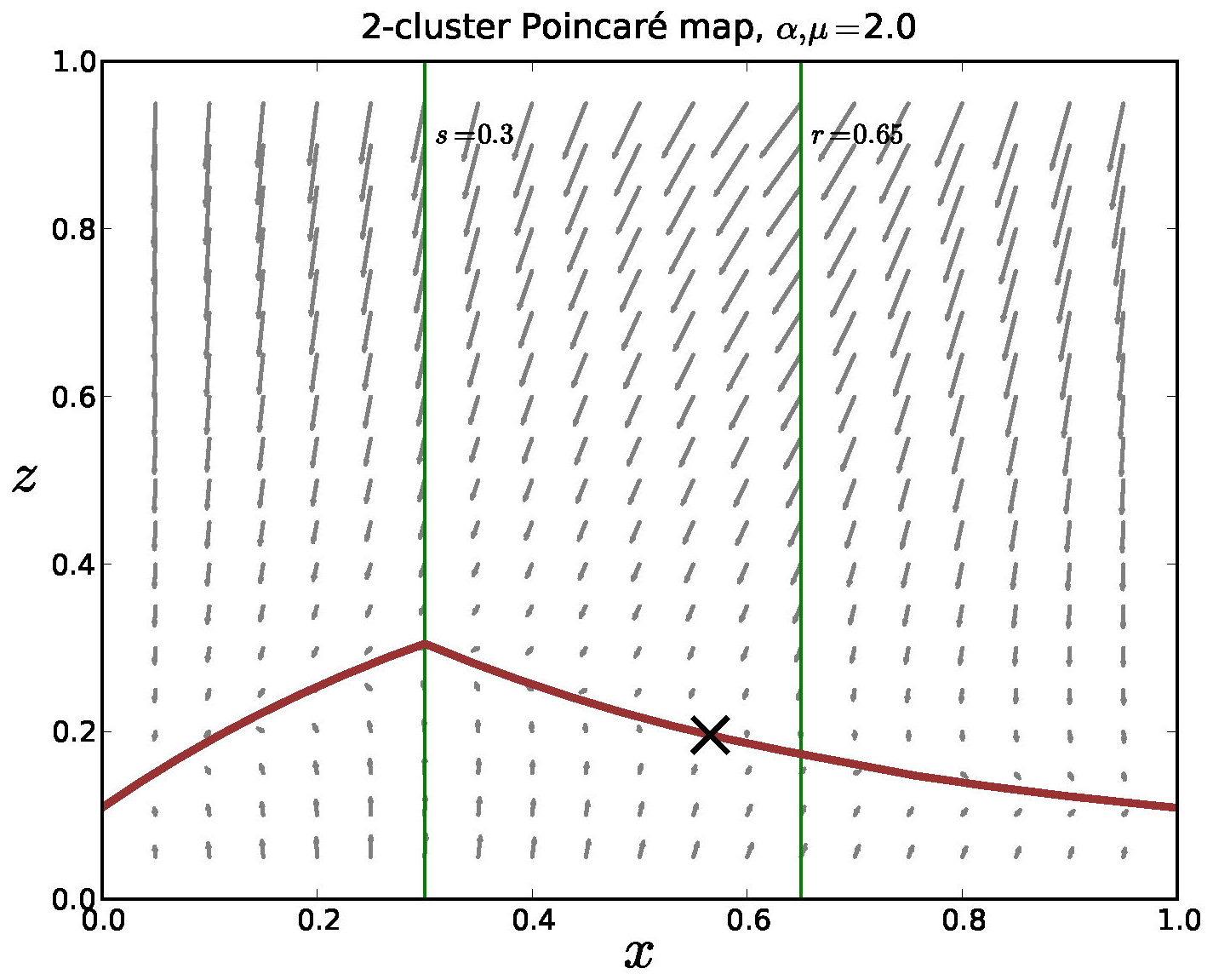
Figure 12. The Poincaré map for the mediated model with negative feedback, 2 clusters and \(\alpha = \mu = 2\). The equations are strongly contractive in the \(z\)-direction and there is a lower dimensional invariant manifold in the return map. We note that analysis is nontrivial since the model is only piecewise smooth and it appears that this manifold is Lipschitz, but not differentiable.

In Figure 13 we compare stability regions predicted in section 2.1 with the model (1) and the mediated model (3). Observe that for the number of clusters realized in simulations is nearly always the same.

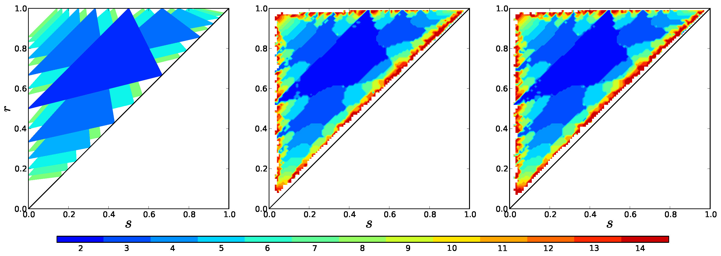
Figure 13. Theoretical stability regions compared with the number of clusters that form in simulations of the basic model (1), and the mediated model (3) with parameters \(\alpha = \mu = 720\) (right) as a function of the parameters \(r\) and \(s\). In all of these \(f(I) =- I\).

In [16] we investigated the possibility that YMO and CDC clustering of cells could be due to an interplay between near-critical metabolism and cell cycle checkpoints. A checkpoint is a position in the cell cycle where further progress may be stopped, e.g., because of insufficient resources. We construct a model of that incorporates checkpoint gating and metabolic mode switching that are triggered by resource thresholds. We investigated the model analytically and proved that there exist open sets of parameter values for which the model possesses stable periodic solutions that exhibit metabolic oscillations with cell cycle clustering. Simulations of the model give evidence that such solutions exist for large sets of parameter values. This demonstrates that checkpoint gating coupled with resource criticality can be a robust mechanism for producing the phenomena observed in experiments.

In [10] we considered the model (1) except with a small gap included between the \(R\) and \(S\) regions. The gap is intended to mimic a delay between production and action of the signaling agent(s) responsible for feedback. The time scales of many of the processes necessary for signaling, such as metabolites passing through the cell membrane are known and are small compared with the period of YMO oscillations. We found that a small gap does not greatly effect the number of clusters that form (it causes small perturbations in the boundaries of parameter regions where different numbers of clusters are stable). However, we found that a gap enhances the stability of stable clusters. In Figure 14 we investigated the convergence of a solution to a stable 4 cluster solution, comparing the model with and without a gap.

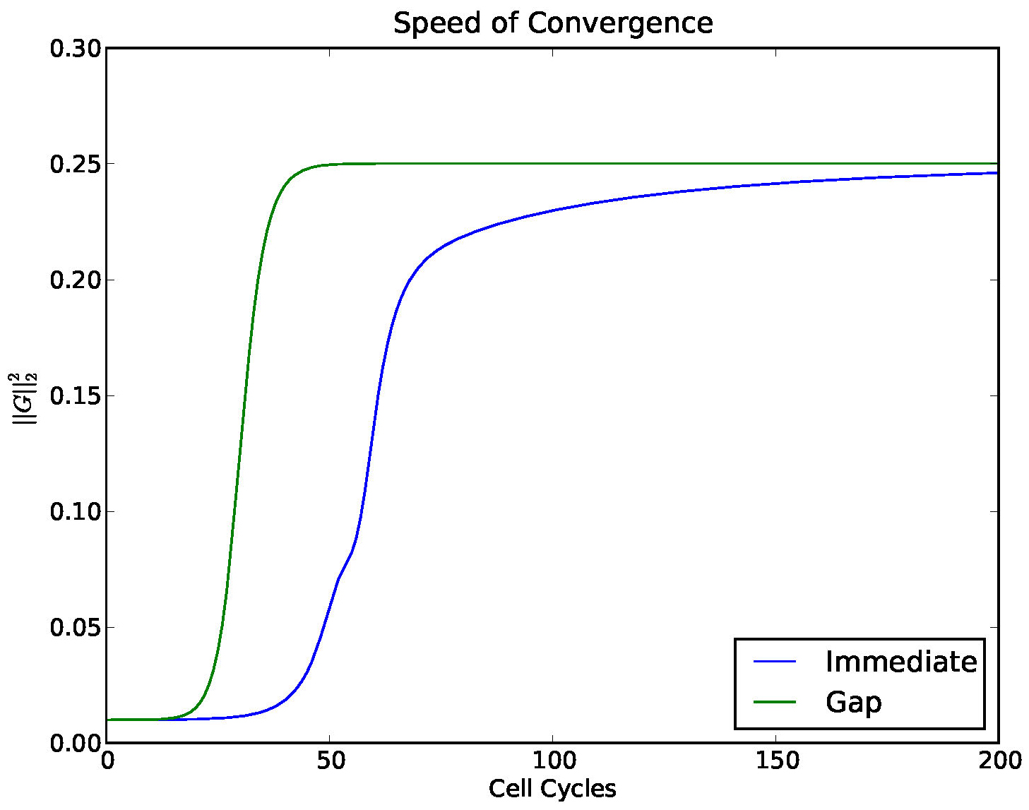
Figure 14. Convergence to a 4-cyclic solution comparing the model (1) with a gap and without. A gap (which mimics a delay) enhances the stability of stable clusters.

Uneven clusters

In all of the above, we considered \(k\) clusters with \(n/k\) cells in each cluster, i.e., evenly distributed clusters.

What about uneven clusters? Can clusters be unequal?

Suppose that for a certain set of parameters the 2-cyclic solution is asymptotically stable. What happens if we make one cluster bigger than the other? Let \(0 < a < 1\) denote the fraction of cells in the smaller cluster.

It turns out that uneven clusters are locally asymptotically stable in the clustered subspace.

Theorem 3. Let \(\alpha = f(a)\) and \(\beta = f(1-a)\) for \(a < 1/2\) and \(\beta < \alpha < 0\). Then for \(r-s \le 1/2\), within the subspace of two cluster solutions with weightings \(a\) and \(1-a\), there exists a unique, attracting periodic orbit for which the two clusters are distinct. The synchronized solution is a repelling periodic orbit in this subspace.

How do cell actually distribute themselves into two clusters? In Figure 15 we plot the results from 1000 simulations of 1000 cells starting from random initial conditions. We use the model (1) with \(f(I) = -.6 I\), \(s = 0.4\), and \(r = 0.65\). For these parameter values, the 2-cyclic solution is stable. After the simulation runs for about 100 cycles, we identify clusters, count the cells in each cluster and find the absolute difference. In the figure we plot a histogram of the distribution of \(|\)differences\(|\) in # of cells/cluster.

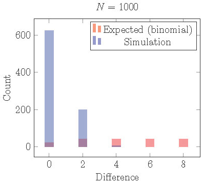
Figure 15. Distribution of cells into two clusters from simulations staring with random initial conditions compared the distribution that would be expected from independent random processes (binomial distribution). Cells are much more equally distributed than they should be. This can be explained by loss of local stability in the full phase space.

Theorem 3 is concerned with local stability in the clustered subspace. With equal clusters, subspace stability implies full stability [17], but we have no such result in the case of uneven clusters. In fact, we have shown [19] the following which explains the tightly even distribution of cells into clusters seen in Figure 15.

Theorem 4. In the full phase space, local stability is lost when clusters are not equal.

However, for the model with an included gap we find the following.

Theorem 5. With a gap, if a periodic solution with uneven clusters is locally asymptotically stable in the 2 cluster subspace then it is locally asymptotically stable in the full phase space.

In other words, unequal clusters can be locally asymptotically stable. If we repeat the simulations illustrated in Figure 15, but with a small gap, then we obtain Figure 16. With a small gap, the uneven 2 cluster solution is locally stable, but clusters are still more evenly distributed than expected from assignment by an independent random process.

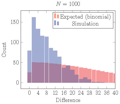
Figure 16. Distribution of cells into two clusters from simulations with a gap staring from random initial conditions. Comparing with the distribution that would be expected from independent random processes (binomial distribution), cells are still more equally distributed than they should be although uneven clusters are locally stable.

In order to understand this, it is necessary to look not only at local dynamics, but also at global dynamics. In Figure 17 we consider the effects of two large clusters in a stable periodic orbit on the dynamics of a single cell. The red dots represent the Poincaré map of a single cell from various initial conditions (horizontal axis). For some initial conditions the single cell will eventually be attracted to cluster 1 and for others it is attracted to cluster 2. The parameter \(a\) represents the fraction of cells in cluster 1 (at \(x=0\)). Solid black dots indicate the stable positions of the large clusters.

We observe in Figure 17 that making clusters uneven shifts the basins of attraction of the clusters. When the clusters have the same number of cells, then the sizes of the basins of the two clusters are nearly equal. But, as one cluster becomes larger, its basin becomes smaller, while the basin of the smaller cluster becomes larger. Thus as clusters are forming, division of cells into clusters is not independent of previous assignments. Cells will be more likely to join a smaller cluster than a larger one.

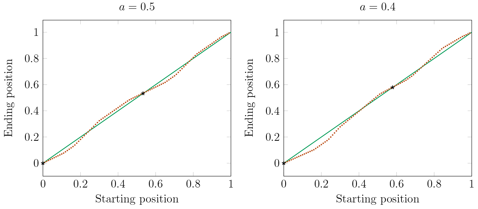
Figure 17. For \(a = .5\) the basins of the two clusters are nearly equal. For \(a = .4\) and smaller, the small cluster has a much larger basin.

Conclusions about Unequal Clusters

 

• Clustering is a robust phenomenon for Negative Feedback.
• Stable clustering requires interaction among clusters.
• Interaction favors equal clusters.
• Global, not Local, dynamics have a large influence.

We think that this is a fairly general principle: systems that form temporal clusters via non-local coupling tend to form nearly equal clusters.

References

[1]   B. Bárány, G. Moses, and T. Young, Instability of the Steady State Solution in Cell Cycle Population Structure Models with Feedback, to appear in J. Math. Biology, doi: 10.1007/s00285-018-1312-0.

[2]   E. Boczko, C. Stowers, T. Gedeon, and T. Young, ODE, RDE and SDE Models of Cell Cycle Dynamics and Clustering in Yeast, J. Biolog. Dyn., 4 (2010), pp. 328--345.

[3]   N. Breitsch, G. Moses, T. Young, and E. Boczko, Cell Cycle Dynamics: Clustering is Universal in Negative feedback systems, J. Math. Biology, 70 (5), 2015, pp. 1151--1175, doi: 10.1007/s00285-014-0786-7.

[4]   R. Buckalew, Cell Cycle Clustering and Quorum Sensing in a Response / Signaling Mediated Feedback Model, DCDS B, 19 (4), 2014, pp, 867--881.

[5]   A. J. Burnetti, M. Aydin, and N. E. Buchler, Cell cycle Start is coupled to entry into the yeast metabolic cycle across diverse strains and growth rates, MBoC, 27 (2016), pp. 64--74.

[6]   S. De Monte, F. d'Ovidio, S. Danø, and P. G. Sørensen, Dynamical Quorum Sensing: Population Density Encoded in Cellular Dynamics, PNAS, 104 (2007), pp. 18377--18381.

[7]   O. Diekmann, H. Heijmans, and H. Thieme, On the stability of the cell size distribution, J. Math. Biol., 19 (1984), pp. 227--248.

[8]   R. K. Finn and R. E. Wilson, Population dynamic behavior of the Chemostat system, Agric. Food Chem., 2 (1954), pp. 66--69.

[9]   B. Futcher, Metabolic cycle, cell cycle and the finishing kick to start, Genome Biol., 7 (2006), pp. 107--111.

[10]   X. Gong, R. Buckalew, T. Young, and E. Boczko, Cell Cycle Feedback Model with a Gap, J. Biol. Dynamics, 8 (2014), pp. 79--98, doi: 10.1080/17513758.2014.904526.

[11]   X. Gong, G. Moses, A. Neiman, and T. Young, Noise-induced dispersion and breakup of clusters in cell cycle dynamics, J. Theor. Biol., 335 (2014), pp. 160--169, doi: 10.1016/j.jtbi.2014.03.034.

[12]   K. Hannsgen and J. Tyson, Stability of the steady-state size distribution in a model of cell growth and division, J. Math. Biol., 22 (1985), pp. 293--301.

[13]   M. A. Henson, Cell ensemble modeling of metabolic oscillations in continuous yeast cultures, Comput. Chem. Engin., 29 (2005), pp. 645--661.

[14]   R. R. Klevecz and D. Murray, Genome wide oscillations in expression, Molec. Biol. Rep., 28 (2001), pp. 73--82.

[15]   M. T. Kuenzi and A. Fiechter, Changes in carbohydrate composition and trehalose activity during the budding cycle of Saccharomyces cerevisiae, Arch. Microbiol., 64 (1969), pp. 396--407.

[16]   L. Morgan, G. Moses, and T. R. Young, Coupling of the Cell Cycle & Metabolism in Yeast Cell-Cycle-Related Oscillations via Resource Criticality and Checkpoint Gating, Lett. BioMath., 5 (2018), doi: 10.1080/23737867.2018.1456366.

[17]   G. Moses, Dynamical Systems in Biological Modeling: Clustering in the Cell Division Cycle of Yeast, PhD thesis, Ohio University, 2015.

[18]   J. B. Robertson, C. C. Stowers, E. M. Boczko, and C. H. Johnson, Real-time luminescence monitoring of cell-cycle and respiratory oscillations in yeast, PNAS, 105 (2008), pp. 17988--17993.

[19]   J. Rombouts, K. Prathom, and T. Young, Cells in Temporally Clustered Solutions Prefer to be Equidistributed, in preparation.

[20]   M. Rotenberg, Selective synchrony of cells of differing cycle times, J. Theor. Biol., 66 (1977), pp. 389--398.

[21]   K. Prathom, Ph.D. dissertation, Ohio University, in preparation.

[22]   N. Slavov and D. Botstein, Coupling among growth rate response, metabolic cycle, and cell division cycle in yeast, Molecular Biology Cell, 22 (2011), pp. 1999--2009.

[23]   C. Stowers and E. M. Boczko, Extending cell cycle synchrony and deconvolving population effects in budding yeast through an analysis of volume growth with a structured Leslie model, JBiSE, 3 (2011), pp. 987--1001.

[24]   C. Stowers, T. Young, and E. Boczko, The Structure of Populations of Budding Yeast in Response to Feedback, Hypoth. Life Sciences, 1 (3), 2011, pp. 71--84.

[25]   K. Von Meyenburg, Stable synchronous oscillations in continuous cultures of S. cerevisiae under glucose limitation, in B. Chance (Ed) Biological Biochemical Oscilllators, Academic Press, NY, 1973.

[26]   T. Young, B. Fernandez, R. Buckalew, G. Moses, and E. Boczko, Clustering in Cell Cycle Dynamics with General Responsive/Signaling Feedback, J. Theor. Biol., 292 (2012), pp. 103--115.