History and Origins of the Korteweg-de Vries Equations Eduard de Jager Korteweg-de Vries Institute University of Amsterdam, the Netherlands (translated from Dutch by Hinke Osinga, University of Bristol, UK)
Professor Eduard de Jager.

Introduction

Korteweg and De Vries gained international recognition for their model equation of shallow-water waves that now bears their name. However, their fame rose only seventy years after the journal publication on the Korteweg-de Vries (KdV) equation, caused by a rediscovery of the KdV equation by Zabusky and Kruskal [23] and the many applications that followed [9].

The mathematical literature usually refers to a simplified form of the KdV equation, but there is actually little difference with the formulations given in the PhD thesis of De Vries from 1894 [22] or the famous paper by Korteweg and De Vries in the Philosophical Magazine of 1895 [12]. Historically, however, the origins of the KdV equation are to be found much earlier, starting with the experiments of Scott Russell in 1834 [21] and the subsequent theoretical research, mainly by Boussinesq in 1871-1877 [1]-[4], Raleigh (Strutt, J.W.) in 1876 [18], and Saint Venant in 1885 [20]. This article considers aspects of the research by Boussinesq, on the one hand, and by Korteweg and De Vries, on the other hand, particularly focusing on the most accessible paper by Boussinesq [3] and the paper in the Philosophical Magazine of Korteweg and De Vries [12]. As we shall see, it is Boussinesq who deserves the honour of having formulated the first satisfactory mathematical description of long waves and is, therefore, actually the true discoverer of the KdV equation, albeit in a disguised way; see also R. Pego [17]. For many historical details, including later developments, the reader is referred to A.C. Newell [15], R.K. Bullough [6], J.W. Miles [14], O. Darrigol [7], and KdV'95 [7].

Problem formulation

In 1834 the Scottish naval architect Scott Russell on horseback followed a towboat, pulled by a pair of horses along the Union Canal, connecting Edinburgh and Glasgow. The boat was suddenly stopped in its speed -- presumably by some obstacle -- but not the mass of water that it had put in motion. Scott Russell observed a very peculiar phenomenon: a nice round and smooth wave -- a well-defined heap of water -- loosened itself from the stern and moved off in forward direction without changing its form with a speed of about eight miles per hour; the wave was about thirty feet long and one or two feet high. He followed the wave on his horse and after a chase of one or two miles he lost the heap of water in the windings of the channel [21]. Many a physicist would not be inclined to analyze this phenomenon and leave it as it was, but Scott Russell recognised the peculiarity of the phenomenon in this seemingly ordinary event. He designed experiments generating long waves in long shallow basins filled with a layer of water and he investigated the phenomenon he had observed. 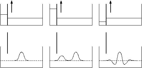He studied the form of the waves, their speed of propagation and stability. A schematic view of these experiments is shown in Figure 1. For a detailed historical study of Scott Russell's work we refer to the overview paper by R.K. Bullough [6].

 

Figure 1: Schematic view of the experiments by Scott Russell; adapted from M. Remoissenet [19].

In the 19th century in England and France there existed a rich tradition in the mathematical description of hydrodynamic phenomena, in particular of wave motions in incompressible fluids without friction; famous names are Airy, Stokes, Rayleigh, Lamb, Lagrange, Saint Venant, and Boussinesq, to name a few. Scott Russell challenged the mathematical community to prove theoretically the existence of his solitary wave and to give an a priori demonstration a posteriori. His challenge did not fail to have an effect. From a mathematical and physical point of view he asked to show the existence of a stable solitary wave that propagates without changing form. In stark contrast with the experimental results of Scott Russell, Airy was of the opinion that this was not possible: a propagating wave would necessarily be steeper at the front and less steep at the back; he was supported in this view by Lamb (1879), Bassett (1888) and McCowan (1892); see [12,22]. Initially, Stokes objected to the well-defined heap of water, because he believed that the only stable wave should be sinusoidal, but later he admitted that he was mistaken.

The a priori demonstration a posteriori, as requested by Scott Russell, was first provided by Boussinesq [1]-[4] in 1871-1877, some time later by Raleigh [18] in 1876, and in order to remove all existing doubts over the existence of the solitary wave, by Korteweg and De Vries [12,22] in 1894. In many ways, Rayleigh used the same methods in his mathematical analysis as Boussinesq and later Korteweg and De Vries. Since Rayleigh's explanation is less detailed, we will not consider it here; see [10] instead.

The equations of Boussinesq and Korteweg-de Vries

The derivations of the equations of Boussinesq and of Korteweg and De Vries are very similar. Both authors consider long waves in a shallow basin with rectangluar cross section; the fluid is assumed incompressible and rotation free, and there is no friction, also not along the boundaries of the basin.

Boussinesq

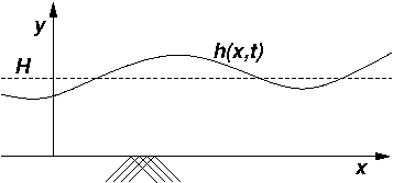
Boussinesq introduces coordinates \((x, y)\) that represent the position of a fluid particle at time \(t\); the pressure in the fluid is denoted \(p\), its density \(\rho\), and the velocity vector \((u, v)\). The height of the water in equilibrium is denoted by the constant \(y = H\) and the wave surface by the function \(y = H + h(x, t)\), where the amplitude \(h\) of the wave is small compared with \(H\); see Figure 2. Finally, he assumes that the wave length is large with respect to \(H\).

 

Figure 2: Mathematical representation of the wave surface.

Since the fluid is rotation free the velocity vector is equal to the gradient of a scalar field, the so-called velocity potential \(\phi(x, y, t)\). Incrompessibility implies that the velocity potential satisfies Laplace's equation, so that we have the series expansions:

\(\phi\)	\(=\)	\( \int f \; dx - \frac{1}{2!} y^2 \frac{\partial f}{\partial x} + \frac{1}{4!} y^4 \frac{\partial^3 f}{\partial x^3} - \dots,\)	(1)
\(u\)	\(=\)	\(\frac{\partial \phi}{\partial x} = f - \frac{1}{2!} y^2 \frac{\partial^2 f}{\partial x^2} + \frac{1}{4!} y^4 \frac{\partial^4 f}{\partial x^4} - \dots,\)
\(v\)	\(=\)	\(\frac{\partial \phi}{\partial y} = -y \frac{\partial f}{\partial x} + \frac{1}{3!} y^3 \frac{\partial^3 f}{\partial x^3} - \frac{1}{5!} y^5 \frac{\partial^5 f}{\partial x^5} + \dots,\)

where \(f\) is an as yet unknown function of \(x\) and \(t\) that slowly varies with \(x\) (the waves are long with respect to \(H\)). The boundary condition \(v = 0\) at \(y = 0\) is satisfied and the boundary condition on the wave surface can be derived from the equations of motion and the kinematic equation.

Integration of equation (1) leads to the Bernoulli equation

where \(g\) is the gravitational acceleration constant and \(\chi\) is an arbitrary function that only depends on \(t\). If the constant atmospheric pressure is \(p_0\) then we also have

and elimination of \(p/\rho\) gives

\(\frac{\partial \phi}{\partial t} + \frac{1}{2} \left( u^2 + v^2 \right) + g h = \chi(t) - g H - \frac{p_0}{\rho} =: \tilde{\chi}(t).\)

(2)

Finally, if we assume that the fluid is at rest for \( x \to \infty\) (or \( x \to -\infty\)), the following boundary condition holds for the wave surface:

\(\frac{\partial \phi_s}{\partial t} + \frac{1}{2} \left( u_s^2 + v_s^2 \right) + g h = 0,\)

(3)

where the subscript \(s\) indicates that for \(y\) the value \(y = H + h(x, t)\) was taken. A second boundary condition follows from the kinematic equation

\( v_s = \frac{d h}{d t} = \frac{\partial h}{\partial t} + u_s \frac{\partial h}{\partial x}.\)

(4)

By expanding \(\phi_s\) and relations (3) and (4) in powers of \((H + h)\) up to terms of order \(O(h^2)\), and after elimination of \(\phi_s\), \(u_s\), and \(v_s\), Boussinesq obtains the following equation for the wave surface that is named after him:

\(\frac{\partial^2 h}{\partial t^2} = g H \frac{\partial^2 h}{\partial x^2} + g H \frac{\partial^2}{\partial x^2} \left( \frac{3 h^2}{2 H} + \frac{H^2}{3} \frac{\partial^2 h}{\partial x^2} \right).\)

(5)

This equation already gives a better approximation than the one given by Lagrange in 1786, namely the wave equation

with general solution \(h(x, t) = h_1(x - \sqrt{g H} t) + h_2(x + \sqrt{g H}t)\).

Boussinesq subsequently restricts his analysis to waves that propagate in the direction of the positive \(x\)-axis, that is, in the Lagrange approximation, waves of the form \(h(x, t) = h_1(x - \sqrt{g H} t)\), with wave speed \(\omega_1 = \sqrt{g H}\).

One can obtain a different form of the differential equation (5) by utilizing the conservation law

\(\frac{\partial h}{\partial t} + \frac{\partial}{\partial x}(\omega h) = \frac{\partial h}{\partial t} + \omega \frac{\partial h}{\partial x} + h \frac{\partial \omega}{\partial x} = 0,\)

(6)

where \(\omega\) is the wave speed. Substitution in (5) and integration with respect to \(x\), while using the condition that \(h\) and all its derivatives with respect to \(x\) go to zero as \( x \to -\infty\), leads to the equation

\(\frac{\partial}{\partial t}(\omega h) + g H \frac{\partial}{\partial x} \left(h + \frac{3 h^2}{2 H} + \frac{H^2}{3} \frac{\partial^2 h}{\partial x^2}\right) = 0.\)

(7)

Using (6) we can write this expression as

Without changing the order of the approximation, we may replace \(\partial / \partial t\) with \(-\sqrt{g H} \partial / \partial x\), so that after integration with respect to \(x\), we obtain the following important formula for the wave speed:

\(\omega = \sqrt{g H} + \sqrt{g H} \left(\frac{3 h}{4 H} + \frac{H^2}{6 h} \frac{\partial^2 h}{\partial x^2} \right).\)

(8)

Substituting this value for \(\omega\) into the relation

where \(d h / d t = \partial h / \partial t + \omega \partial h / \partial x\) is the total differential with respect to \(t\), we obtain an alternative formulation of (7), namely

If we introduce the new variable \(\sigma\) with the definition \(h \; dx = -d \sigma\), this is equivalent to:

\(\frac{d h}{d t} = \frac{1}{4} \sqrt{\frac{g}{H}} \frac{\partial}{\partial \sigma} \left[h^3\left\{1+\frac{2H^3}{3}\frac{\partial}{\partial \sigma}\left(\frac{\partial h}{\partial \sigma}\right)\right\}\right].\)

(9)

Boussinesq does not immediately substitute (8) into (6); had he done this, the result would have become

\(\frac{\partial h}{\partial t} + \sqrt{\frac{g}{H}} \frac{3}{2} \frac{\partial}{\partial x}\left(\frac{2}{3}H h + \frac{1}{2} h^2 + \frac{H^3}{9} \frac{\partial^2 h}{\partial x^2} \right) = 0,\)

(10)

which is the KdV equation "avant la lettre" and only differs from the well-known KdV equation because the coordinates \((x, t)\) refer to a fixed frame, while Korteweg and De Vries used a moving frame. Boussinesq has given another derivation of (10) in a footnote on page 360 of his 680-pages Mémoire "Essai sur la théorie des eaux courantes" [4]. He does not use the wave speed \(\omega\) explicitly, but it can easily be obtained from substitution of (6) in (10); see also R. Pego [17]. Finally, (8) implies that the wave speed varies pointwise, which means that one would expect the propagating wave to change form; this was the subject of the discussion that followed after the discovery of the stationary wave by Scott Russell.

Korteweg and De Vries

Korteweg and De Vries follow the same theoretical arguments as Boussinesq and start with the same boundary value problem. A difference in their treatise is that they take surface tension into account so that the Bernoulli equation (2), when applied to the wave surface, becomes

A second more important difference is that Korteweg and De Vries differentiate this boundary condition with respect to \(x\), which removes the dependence on the arbitrary choice of the function \(\tilde{\chi}\), so that the theory can also be applied to periodic wave motions that do not vanish for \(x \to \pm \infty\); see the section on the periodic stationary wave.

A third difference in the derivation of the differential equation is the wave speed \(\omega\) as a function of \(h(x ,t)\). A wave that is propagating to the right can be stopped approximately by letting the fluid move in the opposite direction, or equivalently, by introducing a moving coordinate frame that moves to the right, initially with uniform speed \(\sqrt{g H}\), and more accurately with speed \(\sqrt{g H} - \alpha \sqrt{g / H}\), where \(\alpha\) is a constant of the same order as \(h(x,t)\) that is to be determined. In this moving frame

\(\xi = x - \left(\sqrt{g H} - \alpha \sqrt{\frac{g}{H}}\right) t, \quad \tau = -t\)

(11)

the differential equation for the wave surface by Korteweg and De Vries becomes

\(\frac{d h}{d \tau} = \frac{3}{2} \sqrt{\frac{g}{H}} \frac{\partial}{\partial \xi}\left(\frac{h^2}{2} + \frac{2 \alpha h}{3} + \frac{\sigma}{3} \frac{\partial^2 h}{\partial \xi^2}\right).\)

(12)

Here, the parameter \(\sigma\) is defined as

with \(T\) the surface tension of the wave surface, which was not taken into account by Boussinesq. Equation (12) is the original KdV equation, as it appeared for the first time in the PhD thesis of De Vries. For \(T = 0\) this equation is equivalent to (10), from which it can be derived by applying the coordinate transformation (11).

The long solitary wave

If we assume that a solitary wave exists then the equivalence of (10) and (12) implies that both theories lead to the same formulation of the surface wave in stationary state. For such a wave all points on its surface must have the same propagation speed so that \(\omega\) must be constant. Using \(\omega = \sqrt{g H} +\) const\(=: \sqrt{g H} + \frac{1}{2} \sqrt{g / H} , h_1\) in (8), we obtain

Under the specific assumption that \(h \to 0\) and \(\partial h / \partial x \to 0\) as \(x \to -\infty\) we get

\(\left( \frac{\partial h}{\partial x} \right)^2 = \frac{3 h^2 (h_1 - h)}{H^3},\)

(13)

and the positive solution becomes

\(h(x, t) = h_1,\) sech\(^2 \left(\sqrt{\frac{3 h_1}{4 H^3}} (x - \omega t)\right)\)

(14)

with

\(\omega = \sqrt{g H} + \frac{h_1}{2} \sqrt{\frac{g}{H}}.\)

(15)

Equation (13) implies that the amplitude of the wave is \(h_1\) and (15) shows, furthermore, that the wave speed increases with the amplitude of the wave. This means that, when there are several different solitary waves of the form (14), higher waves that start behind smaller ones will overtake them. Since there can be no change in shape, the solitary waves behave like a row of rolling marbles, where the faster marbles carry over their impulses to the slower marbles. This is the reason why Zabusky and Kruskal called such waves solitons [23]. For an explicit calculation of this behaviour the interested reader may consult [8, part II, 3.5]. Equations (14)-(15) were also derived by Rayleigh, but he attributes the credit to Boussinesq [18].

Korteweg and De Vries do not have an explicit expression for the wave speed. However, for a stationary wave in the moving frame (11) we have \(\partial h / \partial \tau = 0\) so that equation (12) implies

\(\frac{d}{d \xi} \left(\frac{h^2}{2} + \frac{2 \alpha h}{3} + \frac{\sigma}{3} \frac{d^2 h}{d \xi^2} \right) = 0,\)

(16)

where the correction \(\alpha\) of the wave speed \(\sqrt{g H}\) is still unknown. Assuming \(h\), \(d h / d \xi\), \(d^2 h / d \xi^2 \to 0\) as \(\xi \to -\infty\), integration gives

Korteweg and De Vries distinguish the two cases \(\sigma > 0\) and \(\sigma < 0\); we only consider the case \(\sigma > 0\) so that we must have \(2 \alpha < 0\). Let us choose \(2 \alpha = -h_2\), where \(h_2\) is the wave amplitude. Then we get

\(h(\xi) = h_2\) sech\(^2 \left(\sqrt{\frac{h_2}{4 \sigma}} \xi \right).\)

(17)

If \(T = 0\) then \(\sigma = \frac{1}{3} H^3\) and (17) becomes

\(h(\xi) = h_2\) sech\(^2 \left(\sqrt{\frac{3 h_2}{4 H^3}}\xi \right),\)

(18)

which corresponds to equation (14) of Boussinesq. The wave speeds are also the same, namely, using (11), we have

This approximation of the wave speed, which improves the formula of Lagrange, was verified experimentially already in 1844 by Scott Russell. Korteweg and De Vries also consider negative amplitudes and easily show that such waves exist if \(H < \sqrt{3 T/(\rho g)}\), that is, approximately for water with \(H < \frac{1}{2}\) cm.

The periodic stationary wave

The stationary wave surface satisfies equation (16), but the theory of Korteweg and De Vries does not require \(h\), \(d h / d \xi\), \(d^2 h / d \xi^2 \to 0\) for \(\xi \to +\infty\). Therefore, they do not need this assumption. Integrating (16) twice leads to

and

\(c_2 + 6 c_1 h + h^3 + 2 \alpha h^2 + \sigma \left( \frac{d h}{d \xi} \right)^2 = 0,\)

(19)

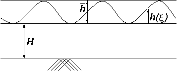
where \(c_1\) and \(c_2\) are integration constants. If we assume that the \(y\)-coordinate at the minimum of the wave surface takes the value \(H\) then the stationary wave surface satisfies \(y = H + h(\xi)\), with \(d h/ d \xi = 0\) and \(d^2 h / d \xi^2 > 0\) for \(h = 0\); see also Figure 3. Hence, \(c_2 = 0\) and if we further assume \(\sigma > 0\), we also have \(c_1 < 0\).

Figure 3: Formulation for wave with minimal height \(H\).

This implies that the equation \(\mu^2 + 2 \alpha \mu + 6 c_1 = 0\) has a positive root \(\bar{h}\) and a negative root \(-k\), so that (19) reduces to

\(\frac{d h}{d \xi} = \pm \sqrt{\frac{1}{\sigma} h (\bar{h} - h) (h + k)}, \quad \bar{h} > 0, \quad k > 0.\)

(20)

Using the substitution \(h = \bar{h} cos^2 \chi\) we obtain the periodic solution

\(h(\xi) = \bar{h},\) cn\(^2 \left(\sqrt{\frac{\bar{h} + k}{4 \sigma}} \xi \right),\)

(21)

where cn denotes one of the Jacobian elliptic functions with modulus \(M = \bar{h} / (\bar{h} + k)\) and period

Korteweg and De Vries called such waves cnoidal waves and the wave surface forms a train of periodic waves with wave length \(4 K \sqrt{\sigma / (\bar{h} + k)}\). If \(k = 0\) and \(M= 1\) then the wave length becomes infinite and one obtains the stationary solitary wave (17); if \(k \to \infty\) and \(M \to 0\) then the result is approximately the sinusoidal wave

where the wave length decreases with increasing \(k\); this corresponds to the result of Stokes [14]. Note that in this case \(h(\xi)\) may be expanded in a Fourier series; this may be the reason why Stokes at first believed that the only permanent wave should be of sinusoidal type. Boussinesq also considered in his Mémoire [4, pp 390-396] the general case of a periodic stationary wave. However, he is forced to use a different set of equations, because his assumption that \(h\) vanishes at infinity does not hold for periodic waves; see also [20]. His result is, in principle, the same as equation (20) but he does not provide an explicit solution. It is the merit of Kortweg and De Vries that they have given a unified treatment of the stationary solitary wave, valid for waves vanishing at infinity as well as periodic waves.

The stability of the stationary solitary wave

The goal of the research by Boussinesq and Korteweg and De Vries was the study of the behavior of long waves on the surface of a fluid in a shallow basin. In general, wave propagation involves a change of form, but by definition this does not occur in the case of a steady wave and so the question arises why the steady solitary wave is stable and an exception to the rule. For the possible existence of the steady wave further investigation is required, in particular with regard to the "parameters" determining the stable behavior. This has been carried out by Boussinesq and Korteweg and De Vries in quite different ways. The presence in (7) and (12) of the non-linear term \(h , d h / d \xi\) and the dispersion term \(\frac{1}{3}\sigma , \partial^3 h / \partial \xi^3\) is already an indication for a possible balance, furthering the stability of the wave.

Stability in the theory of Korteweg and De Vries

Korteweg and De Vries consider a wave form close to that of the steady solitary wave

\(h(\xi, 0) = \bar{h},\) sech\(^2(p \xi),\)

(22)

where \(\bar{h}\) and \(p\) are as yet arbitrary constants. The deformation of \(h(\xi, \tau)\) is determined by equation (12) and substitution of (22) leads to an equation for the wave surface \(h(\xi, \tau)\) as a function of \(\xi\) and \(\tau\):

\(\frac{\partial h}{\partial \tau} = -3 \sqrt{\frac{g}{H}} \bar{h}p(4\sigma p^2 - \bar{h})\left\{-\mbox{sech}^2(p \xi)+\frac{2(\alpha + 2\sigma p^2)}{3 (4 \sigma p^2 - \bar{h})}\right\}\mbox{sech}^2(p \xi)\mbox{tanh}(p \xi).\)

(23)

If we choose \(\alpha\) and \(p\) such that \(2 (\alpha + 2 \sigma p^2) = 3(4 \sigma p^2 - \bar{h})\), that is \(\alpha = 4 \sigma p^2 - \frac{3}{2}\bar{h}\), then (23) becomes

\(\frac{\partial h}{\partial \tau} = -3 \sqrt{\frac{g}{H}} p \bar{h} (4 \sigma p^2 - \bar{h})\mbox{sech}^2(p \xi) \mbox{tanh}^3(p \xi).\)

(24)

The choices \(p = \sqrt{\bar{h} / (4 \sigma)}\) and \(\alpha = - \frac{1}{2} \bar{h}\) ensure that \(\partial h / \partial \tau = 0\) and we get the steady wave (17).

Further numerical analysis of (24), using Table IX from Traité des fonctions elliptiques (II) by Legrendre [13], shows that, in its course, the wave becomes steeper in front and less steep behind when \(\bar{h} > 4 \sigma p^2\) and, the converse when \(\bar{h} < 4 \sigma p^2\). This result is in contradiction with the assertion of Airy, among others, that a progressive wave always gets steeper in front and less steep behind. This opinion is conceivable given the fact that the KdV equation, when neglecting the dispersion term \(\frac{1}{3} \sigma \partial^3 h / \partial \xi^3\), can be reduced to \(\partial h / \partial \tau + h \partial h / \partial \xi =0\), which implies that particles on the wave surface move faster to the right as they are higher on the wave's crest. In a steady wave, the dispersion term \(\frac{1}{3}\sigma \partial^3 h / \partial \xi^3\) compensates the nonlinear term \(h , \partial h / \partial \xi\).

Stability in the theory of Boussinesq

For studying stability, Boussinesq considers waves with the same energy satisfying

Furthermore, he introduces the functional

which he calls the moment de stabilité. Straightforward calculation shows that \(M\) is a conserved quantity, that is, \(d M / dt = 0\) for any wave satisfying (7) and (8). After the transformation

the expression for \(M\) becomes

Boussinesq uses the well-known Euler-Lagrange method, without a reference, to obtain a condition for \(h(\varepsilon, t)\) such that \(M\) attains an extremal value. The result is

Using \(d \varepsilon = - h^2 \; d x = h \; d \sigma\) or \(h \frac{\partial}{\partial \varepsilon} = \frac{\partial}{\partial \sigma}\) one obtains equation (9) with \(d h / d t = 0\). Therefore, only the stationary solitary wave with given energy \(E\) yields an extremum for \(M\). Variation of \(h\) with \(\Delta h\) gives \(\Delta M > 0\) for all \(h(\varepsilon, t)\), so that \(M\) is a minimum among all waves with given energy, provided the corresponding wave \(h(\varepsilon, t)\) is stationary. The stability of the wave is evident, because also \(\Delta M\) does not depend on \(t\).

We particularly mention this result, because \(M\) inherits several properties from the Hamiltonian that appears in the formulation of the KdV equation as a Hamiltonian system. The theory of continuous Hamiltonian systems has been investigated only recently and the first fundamental results have been established in the late sixties by P. Lax in 1968 [11], Zacharov in 1969 [24], and L.J.F. Broer in 1974 [5]. We further refer to P.J. Olver [16] and E. van Groesen and E.M. de Jager [8, part I, Ch. 1, 2, part II, Ch. 5], where the theory of infinite-dimensional continuous dynamical systems is considered in detail.

The KdV equation can be represented as a Hamiltonian system in the form

where

Here, \(\delta_h ({\mathcal{H}})\) is the variational derivative of the Hamiltonian \({\mathcal{H}}\) and \(\varepsilon\) is a scale parameter. The first term of \({\mathcal{H}}\) is the Hamiltonian for waves in the Lagrange approximation and the second term is the Boussinesq correction, given by \(M\), the moment de stabilité. Hamilton's theory for finite discrete systems dates from about 1835 and it was a century after Boussinesq that this theory has been generalized for continuous systems. By using functionals, Boussinesq has set a first step into the direction of this generalization.

Other interesting topics

We only discussed the most important aspects of the work of Boussinesq and Korteweg and De Vries. The authors further consider in detail the velocity field in the fluid, the paths of the fluid particles, the motion of the centre of gravity of a solitary wave, and a number of characteristic quantities such as the potential and kinetic energy of a wave. Boussinesq ends his article in [3] with a qualitative study of the change of form of long non-stationary waves. Obviously, the wave speed \(\omega\) (8) is important here. The signs of \(h\) and \(h_{xx}\) determine the relative speed of a particle on the wave surface with respect to the base speed \(\sqrt{g h}\). Boussinesq gives heuristic arguments for the possibility that a positive solitary wave splits into several other positive solitary waves, and that negative solitary waves cannot occur (NB \(T = 0\)).

Korteweg and De Vries wanted to show that their approximation of the surface of a steady wave may be improved indefinitely, resulting in a convergent series. Their starting point is the first approximation given in (21) and the equalities

and

where \(f\) is defined in (1); see also equation (20). The coefficients \(a\), \(b\), \(c, \dots\) and \(q\), \(r\), \(s, \dots\) are determined by the boundary conditions that are imposed on the wave surface. Namely,

and

The result is a series expansion with general term \(O(\bar{h}^m)\). While the calculations are elementary, they are so complicated and tedious that one does not expect them to have received much attention. Even the second approximation following (21) already requires so much effort that it is commendable to content with the first approximation (21) only.

Concluding remarks

It is somewhat surprising that Korteweg and De Vries only cite Boussinesq's short communication in the Comptes Rendus of 1871 [1] and not the extensive papers in the J. Math. Pures et Appl. [3] and the Mémoire [4] that appeared in 1872 and 1877, respectively.

B. Willink (Erasmus University Rotterdam) provided this author with a copy of an abstract written by De Vries of a paper by Saint Venant [20] from 1885. This copy shows that De Vries was certainly aware of the "Essai sur la théorie des eaux courantes." Hence, one may ask why Korteweg and De Vries revisited the research by Boussinesq only in 1894. The answer is clarified in the introduction of their paper in the Philosophical Magazine [12]. They write that Lamb and Basset still believe that propagating waves must change shape, steeper at the front and less steep behind. Furthermore, the research of Boussinesq, Lord Rayleigh, and Saint Venant appear to corroborate this assumption, even though it is difficult to see why the solitary wave would be an exception. Therefore, they decided to re-examine this research. Maybe it was not customary in the nineteenth century, as it is now, to cite all relevant publications by other authors; moreover, communications cannot have been so easy as they are nowadays. Finally, there is a principle difference between the research on stationary waves by Boussinesq and by Korteweg and De Vries: namely, Boussinesq takes the conservation law (6) and the wave speed \(\omega\) (8) as the starting point of his theory, while Korteweg and De Vries consider the famous KdV equation as "This very important equation, to which we shall have frequently to revert in the course of this paper." The presentation of the two treatises differ enormously: Boussinesq is rather elaborate, while Korteweg and De Vries remain direct and to the point.

The honor of the discovery of the mathematical formulation of the stationary solitary wave and, thus, the KdV equation undoubtedly should go to Boussinesq. However, Korteweg and De Vries did add several new aspects to the theory and were instrumental in removing all doubt with respect to the existence of a stationary solitary wave.

The author is indebted to the grandsons of Gustav de Vries for presenting him with a copy of the doctoral thesis of their grandfather and for the records of the handwritten correspondence between Korteweg and De Vries. The author likes to thank dr. B. Willink (Erasmus University, the Netherlands) for discussions on who first discovered the KdV equation and for copies of some of the work of Boussinesq and Saint Venant. He also thanks dr. F. van Beckum (University of Twente, the Netherlands) for a program to illustrate the interaction of solitons and for his help in the preparation of this article. He is very much indebted to dr. H. Osinga of the University of Bristol, who took great care to translate the original Dutch text into English and to publish this historical essay in DSWeb Magazine.

Bibliography

1	Boussinesq, J.: Théorie de l'intumescence liquide appelée "onde solitaire" ou "de translation", se propageant dans un canal rectangulaire; C. R. Ac. des Sci., Paris, 72, pp. 755-759, 1871.
2	Boussinesq, J.: Théorie générale des mouvements, qui sont propagés dans un canal rectangulaire horizontal; C. R. Ac. des Sci., Paris, 73, pp. 256-260, 1871.
3	Boussinesq, J.: Théorie des ondes et des remous qui se propagent le long d'un canal rectangulaire horizontal, en communiquant au liquide continu dans ce canal des vitesses sensiblement pareilles de la surface au fond; J. Math. Pures et Appl. 17, pp. 55-108, 1872.
4	Boussinesq, J.: Essai sur la théorie des eaux courantes; Mémoires présentés par divers savants à l'Ac. des Sci. Inst. Nat. France XXIII, pp. 1-680, 1877.
5	Broer, L.J.F.: On the Hamiltonian theory of surface waves; Appl. Sci. Res. 30, pp. 430-446, 1974.
6	Bullough, R.K.: "The Wave", "Par Excellence", the Solitary Progressive Great Wave of Equilibrium of the Fluid; An Early History of the Solitary Wave; Solitons: Springer Series in Nonlinear Dynamics, Proceedings, ed. Lakshmanan; pp. 7-42, 1988.
7	Darrigol, O.: The Spirited Horse, the Engineer and the Mathematician; Water Waves in Nineteenth-Century Hydrodynamics; Arch. Hist. Exact Sci. 58, pp. 21-95, 2003.
8	Groesen, E. van, Jager, E.M. de: Mathematical Structures in Continuous Dynamical Systems, North Holl. Publ., pp. 1-617, 1994.
9	Hazewinkel, M., Capel, H.W., Jager E.M. de, eds.: KdV '95, Proceedings International Symposium; Kluwer Acad. Publ.; Reprinted Acta Applicandae Mathematicae 39, pp. 1-516, 1995.
10	Jager, E.M. de: On the origin of the Korteweg-de Vries equation, arXiv:math.HO/0602661, February 28, 2006.
11	Lax, P.: Integrals of Nonlinear Equations of Evolution and Solitary Waves; C.P.A.M. 21, pp. 467-490, 1968.
12	Korteweg, D.J., de Vries, G.: On the Change of Form of Long Waves Advancing in a Rectangular Canal, and on a New Type of Long Stationary Waves; Phil. Mag. 39, pp. 422-443, 1895.
13	Legendre, A.M.: Traité des Fonctions Elliptiques, Huzard-Courcier, Paris, 1825-1828.
14	Miles, J.W.: The Korteweg-de Vries equation: a historical essay; J. Fluid Mech. 106, pp. 131-147, 1981.
15	Newell, A.C.; Solitons in Mathematics and Physics; SIAM, Reg. Conf. Series in Appl. Math., pp. 1-244, 1985.
16	Olver, P.J.: Application of Lie groups to Differential Equations; 2nd ed., Springer, pp. 1-513, 1993.
17	Pego, R.: Origin of the KdV Equation; Notices of the Amer. Math. Soc. 45, 3, p. 358, 1997.
18	Rayleigh, (Strutt, J.W.); On Waves; Phil. Mag. 1, pp. 257-271, 1876.
19	Remoissenet, M.: Waves Called Solitons, Concepts and Experiments, Springer, pp. 1-236, 1994.
20	Saint Venant, de: Mouvements des molecules de l'onde dite solitaire, propagée à la surface de l'eau d'un canal; C. R. Ac. Sci. Paris 101, pp. 1101-1105, 1215-1218, 1445-1447, 1885.
21	Scott Russell, J.: Report on Waves; Rept. Fourteenth Meeting of the British Association for the Advancement of Science; J. Murray, London, pp. 311-390, 1844.
22	Vries, G. de: Bijdrage tot de Kennis der Lange Golven, PhD Thesis, Universiteit van Amsterdam, 1894.
23	Zabusky, N.J., Kruskal, M.D.: Interaction of "Solitons" in a collisionless plasma and the recurrence of initial states; Phys. Rev. Letters 15, pp. 240-243, 1965.
24	Zakharov, V.E., Faddeev, L.P.: The Korteweg-de Vries equation: a completely integrable Hamiltonian system; Funct. Anal. Appl. 5, pp. 280-287, 1971.

About the author

The author was born in 1927 and started his mathematical career at the University of Groningen in the Netherlands. In 1953, after his masters degree in mathematics and physics, he joined the National Aerospace Laboratory (NLR) in Amsterdam, an excellent environment to acquire experience in solving initial boundary value problems in models for the flow around wings. To broaden his horizon he accepted in 1960 a position at the Mathematical Centre (CWI) in Amsterdam where he worked in different areas: theory of generalized functions, singular perturbations and applications of mathematics. Shortly after his Ph.D. in 1964 he was appointed as full professor at the University of Twente and he changed this position four years later for a chair at the University of Amsterdam where he served until his retirement in 1992. In between he was a guest professor at the University of Cologne in 1976 and 1992. He enjoys a happy family life with his wife and two sons. In his younger years he was an enthousiastic sailor and nowadays he finds his pleasure in drawing and painting.

Selected publications

1.	Oscillating Rectangular Wings in Supersonic Flow with Arbitrary Bending and Torsion Mode Shapes. Transactions NLR, Amsterdam, XXVI (1959).
2.	Applications of Distributions in Mathematical Physics. Mathematical Centre Tracts 10, Amsterdam, pp 1-182 (1964), Sec. Ed. (1969).
3.	Lorentz Invariant Solutions of the Klein-Gordon Equation. SIAM J. Appl. Math. 15, no 1 (1967).
4.	with W.Eckhaus, Asymptotic Solutions of Singular Perturbation Problems for Linear Differential Equations of Elliptic Type. Arch. Rat. Mech. and Anal. 23, no 1 (1966).
5.	with Jiang Furu, The Theory of Singular Perturbations. Series in Appl. of Math. and Mech. 42, North-Holland Publ. Cy, Amsterdam, pp 1-340 (1996).
6.	with E.van Groesen, Mathematical Structures in Continuous Dynamical Systems. Studies in Math. Phys. 6, North-Holland Publ. Cy, Amsterdam, pp 1-617 (1994).
7.	with S.Spannenburg and M.H.Sitters, Baecklund Transformations of Solutions of Nonlinear Evolution Equations and the Lie-Bianchi Transformation. Physica A 228 (1996).