Ryan Goh, Boston University, Department of Mathematics and Statistics, 111 Cummington Mall, Boston, MA 02215, USA

1. Introduction

The process of spatial growth plays an important role in controlling and mediating pattern formation in a vast array of natural and man-made experimental systems. Examples of the former include digit and tissue patterning in early stage development [17, 34], primodium arrangement near plant meristems [30], or chemical precipitation and deposition in the wake of a traveling reaction front [38]. Examples of the latter include the formation of nanoscale patterns in ion-milling of metallic alloys [25], water-jet cutting and etching [9], chemical evaporation and de-wetting [42, 37], directional quenching of liquid melts [8], and crystallization in liquid crystals [1]. In all these examples, it is of interest how growth can change the resulting pattern in a system.

In this article we give an overview of recent works [2, 3, 11, 13, 14, 15, 32] which seek to mathematically explore and understand this interaction using a simple model for growth known as a quenching heterogeneity. To explore phenomena, we consider the effect of quenching in the Swift-Hohenberg equation, a prototypical pattern-forming system. In this setting, we highlight how techniques from dynamical systems, functional analysis, modulation theory, and numerical continuation reveal a rich set of pattern-forming dynamics. We expect many of the techniques used and phenomena observed here to have bearing in other models for pattern-formation.

The rest of Section 1 reviews some known results on patterns in Swift-Hohenberg, introduces the concept of a quenching heterogeneity, and defines a mathematical object which we use to classify pattern selection. Section 2 gives an overview of different mathematical approaches used to study quenched patterns in various regimes, while Section 3 briefly discusses areas of future work. This article can also be viewed as an advertisement for a somewhat more detailed and comprehensive review paper [12] on this topic. As such we aim to be light on details, and focus on interesting concepts, and phenomena which arise in this setting.

1.1. Patterns in the Swift-Hohenberg equation

The Swift-Hohenberg equation was originally derived to model roll formation in Rayleigh-Bénard convection [36] and has since been used to model patterns in many different physical systems, such as deformation of elastic surface crystals [35], and plant phylotaxis [30]. Indeed this last application motivated Alan Turing to develop a similar equation in unpublished notes [6] done after the seminal work [40] on morphogenisis. The equation, in two spatial dimensions, takes the form

\( u_t = -(1+\Delta)^2 u + \mu u - u^3,\qquad u\in \mathbb{R}, \, (x,y,t)\in\mathbb{R}^2\times\mathbb{R}_+,\qquad \Delta = \partial_x^2+\partial_y^2 \)

(1.1)

where \(u\) is an order parameter, originally representing the deviation from a pure conductive fluid state represented by \(u\equiv0\), and \(\mu\) an onset parameter which measures stability of the pure conductive as the temperature difference is increased. From a phenomenological viewpoint, this equation is arguably the simplest scalar model which forms stable periodic equilibrium solutions via a Turing instability. Such an instability is observed by inserting \(u =\mathrm{e}^{\lambda t + \mathrm{i}(k_xx+k_yy)}\) into the linear part of (1.1) to obtain the linear dispersion relation

\( \lambda = -(1-k^2)^2 + \mu,\quad k := \sqrt{k_x^2+k_y^2} \).

(1.2)

This relates the temporal growth rate \(\lambda\) to the bulk spatial wavenumber \(k\). For \(\mu<0\) all wavenumbers decay, and the equilibrium state \(u\equiv0\) is stable. As \(\mu\) increases through 0, modes \(k\sim 1\) destabilize; see Figure 1.1. Evolving the nonlinear system from small fluctuations of the now unstable equilibrium \(u\equiv0\), unstable modes grow until they are saturated by the cubic nonlinearity. Furthermore, at onset \(0<\mu\ll1\), one can use standard bifurcation or center manifold techniques [16] to show the existence of stationary stripe solutions \(u_p(k x;k)\) which solve

\( 0 = -(1+k^2 \partial_\theta^2) u_p + \mu u_p - u_p^3, \qquad \theta\in[0,2\pi), u(\theta+2\pi;k) = u_p(\theta;k) \).

(1.3)

for a range of wavenumbers \(k\in(k_\mathrm{ex,-},k_\mathrm{ex,+})\). In fact, they take the simple leading order form

\( u_p(k x;k) = \sqrt{\frac{4(\mu - \kappa^2)}{3}} \cos(k x) + \mathcal{O}(|\mu|),\qquad \kappa = 1 - k^2,\qquad \kappa^2\leq \mu \).

(1.4)

These patterns exist for all wavenumbers \(k\in(k_\mathrm{ex,-},k_\mathrm{ex,+})\) with \(k_{\mathrm{ex},\pm}\approx \sqrt{1\pm\sqrt{\mu}}\). Note that since (1.1) is rotationally invariant, stripes of any orientation \(u_p(k_x x + k_y y;k)\) for such \(k\) are also equilibrium solutions. The stability of such stripes is well-characterized. Indeed a temporal center-manifold approach can be used to show that these patterns are stable with respect to co-periodic perturbations, a Fourier-Bloch wave analysis establishes spectral stability to spatially localized perturbations [23], and a renormalization group analysis gives diffusive stability at the nonlinear level [33].

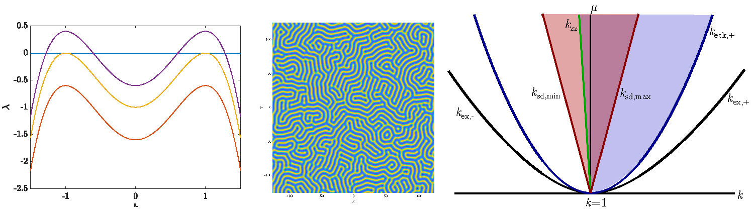
Figure 1.1: Left: linear dispersion relation (1.2) for \(\mu<0\) (orange), \(\mu=0\) (yellow), \(\mu>0\) (purple); Center: Solution of (1.1) with small random initial data and \(\mu = 3/4\), color denotes value of \(u\); Right: Pattern existence and stability domain in \((\mu,k)\sim (0,1)\). Patterns exist above the black curve, are Eckhaus stable above the blue curve, zig-zag stable to the right of the green curve. The red shaded region gives possible wavenumbers for stationary quench in \(1\)-D, while the blue shaded region gives \(2\)-D stability.

1.2. Quenched patterns and the Moduli space

If the trivial state \(u\equiv0\) is perturbed by small white-noise, modes with \(|(k_x,k_x)|\sim1\) of any orientation will be excited, leading to the formation of a defect-laden state with patches of randomly oriented stripes; see Figure 1.1, center plot. Furthermore, one does not have control of the precise wavenumber formed in any given region of the domain. In order to mediate this pattern-forming process and select the wavenumber and orientation of a pattern, one can spatially progressively excite patterns, allowing them only in a subset of the domain which grows as time evolves. This can be modeled by introducing a heterogeneous bifurcation parameter into (1.1)

\( u_t = -(1+\Delta)^2 u + \rho(x,y,t) u - u^3,\qquad \rho(x,y,t) = \begin{cases} \mu,&\qquad (x,y)\in \Omega_t,\\ -\mu,&\qquad (x,y)\in \Omega_t^c, \end{cases},\qquad \mu>0 \),

(1.5)

where \(\Omega_t\subset \mathbb{R}^2\) is a time-dependent expanding domain, with complement \(\Omega_t^c\) and boundary \(\partial\Omega_t\). As \(\partial\Omega_t\) traverses \(\mathbb{R}^2\), it converts \(u = 0\) from a stable to an unstable state so that patterns are only allowed in \(\Omega_t\). Inspired by similar processes in material science [8, 39], we call such a dynamic heterogeneity a quench. Broadly, one is interested in how the geometry and evolution of \(\Omega_t\) affects the type of pattern formed in the wake; see Figure 1.2 for examples with \(\Omega_t = \{ x^2+y^2 < c t\}\) for different radial speeds \(c>0\). We mention similar quenching processes have also been used as an experimental and mathematical model for pattern formation on a growing domain [24, 20]. In particular they model apical growth where material is only added at the boundary of the organism, not in the interior [5]. One could also view this heterogeneity as a dynamic effective boundary condition which enforces spatial decay of solutions outside of \(\Omega_t\).

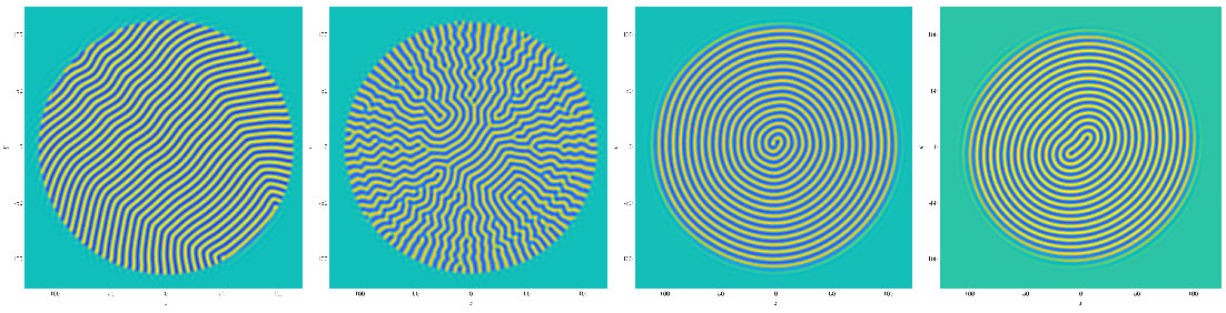
Figure 1.2: Solutions of (1.5) with radial quench, small white-noise initial condition, \(\mu = 3/4\) and \(c =0.05, 0.4, 1,3\) from left to right.

As even the radial quench yields patterns of stunning variety, we consider the simplest possible geometry, a directional quench

\( \Omega_t = \{x-c_x t<0\} \),

(1.6)

where \(\partial\Omega_t\) is a vertical line which rigidly propagates with speed \(c_x\) across the domain. We note such a quenching geometry could also be viewed as the large-radius limit of the radial quench. Figure 1.3 shows the result of simulations seeded with small random fluctuations about the equilibrium state \(u = 0\) for various \(c_x>0\). We qualitatively observe for slow speeds stripes which are perpendicular to the quench interface \(\partial\Omega_t\) are selected, for moderate speeds, stripes oblique to the interface, while for fast speeds, parallel striped patterns are selected. Finally, we find for yet larger speeds, patterns detach from the quench, and invade the now unstable state with a speed less than \(c_x\).

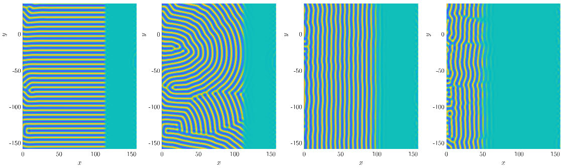
Figure 1.3: Patterns in (1.5) with (1.6), \(\mu = 3/4\), and \(c_x =0.4, 1, 3, 5\) from left, time chosen so \(\partial\Omega_t\) is at \(x\sim110\) for each.

To organize these dynamic phenomena, we consider the simplest pattern-forming front solutions to (1.5). In particular, we study solutions \(u(x,y,t) = u(x - c_x t,k_y (y - c_yt))\) in the co-moving frame variable \(\tilde{x} = x-c_x t\) where the quench is stationary, which are \(2\pi\)-periodic in the co-rotating frame variable \(\tilde{y} =k_y (y - c_y t)\), converge to the trivial state as \(\tilde{x}\rightarrow+\infty\), and to a stripe solution as \(\tilde{x}\rightarrow-\infty\). Here we consider 1:1 resonant solutions so that the temporal frequency \(k_y c_y\) of the solution matches that of horizontal spatial oscillations of the pattern in the co-moving frame, \(k_y c_y = k_x c_x\), and thus the stationary stripe state satisfies \(u_p(k_x x + k_y y;k) = u_p(k_x \tilde x + \tilde y;k)\). In sum, we search for solutions to the following partial differential equation, dropping the tilde notation for simplicity,

\( 0 = -(1+\partial_{x}^2 + k_y^2 \partial_{ y}^2)^2u + \rho( x) u - u^3 + c_x(\partial_x+k_x\partial_y) u \),

(1.7)

\( 0 = \lim_{x\rightarrow -\infty} |u(x,y) - u_p(k_x x + y;k)|,\quad 0 = \lim_{x\rightarrow+\infty} u(x,y),\quad u(x,y+2\pi) = u(x,y) \),

(1.8)

Note in this frame the quench takes the simplified form \(\rho(x) = -\mu\, \mathrm{sign}(x)\). Wishing to relate the asymptotic wavenumbers \((k_x,k_y)\) to the growth speed \(c_x\) we consider the following variety, which we term the Moduli Space,

\( \mathcal{M}:= \{ (k_y,c_x,k_x)\,:\, \) (1.7)-(1.8) has a solution\(\}\).

(1.9)

This object, depicted in Figure 1.4, is a compactified representation of the space of solutions to (1.7)-(1.8) in \((k_y,c_x,k_x)\)-parameter space which classifies patterns in terms of their asymptotic behavior and neglects the behavior of solutions near the quench interface. It also collapses families of \(y\)-translates of a given solution, representing all as a single point. Here points with \(k_x = 0\) correspond to perpendicular stripes, \(k_y,k_x\neq0\) oblique stripes, and \(k_y = 0\) parallel stripes. Arguments using Fredholm theory and group velocities of patterns emanating from the quench can be used to show that \(\mathcal{M}\) can be written locally as a two-dimensional graph in \(k_x\) over \((k_y,c_x)\) near generic points [2, Section 6]. One wishes to understand how the boundaries and geometry of \(\mathcal{M}\) relate to those of the space of solutions to (1.7)-(1.8). Practically, this set can be viewed as a cookbook, allowing experimentalists to understand which patterns can be selected for a given growth speed. Abstractly, it is of interest how \(\mathcal{M}\) varies across different parameter regimes and, more broadly, across different pattern-forming models.

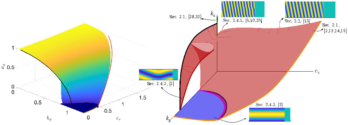
Figure 1.4: Left: numerical continuation of several parts of \(\mathcal{M}\) for \(\mu = 1/4\) (Reproduced from [2, Figure 15]); Right: Schematic plot of Moduli space \(\mathcal{M}\) for (1.7); various regions are labeled with relevant sections below, previous works, and example solution profiles in the co-moving, co-rotating coordinates \((x,y)\); Solid, bold lines give different boundaries of \(\mathcal{M}\) discussed below (see also [2]): all-stripe detachment \((k_y,c_\mathrm{lin}(k_y),k_{x,\mathrm{lin}}(k_y))\) (orange), kink-forming saddle-node \((k_y,c_\mathrm{x,osn}(k_y),k_\mathrm{x,osn}(k_y))\) (red), zig-zag critical \((k_y,c_x = 0,k_\mathrm{x,zz}(k_y))\) (black), oblique reattachment pitchfork \((k_y,c_\mathrm{x,opf}(k_y),0)\) (magenta), perpendicular saddle-node \((k_y,c_\mathrm{x,osn}(k_y),0)\) (blue); range of the strain-displacement relation \(k_x\in \mathrm{Rg}\, g = [k_\mathrm{sd,min},k_\mathrm{sd,max}]\) with \(c_x = k_y = 0\) (green).

2. Overivew of approaches and exploration of different regimes of \(\mathcal{M}\)

We now highlight several methods which have been employed to approximate, construct, and continue solutions in various regimes of \(\mathcal{M}\). The first is the spatial dynamics approach which views (1.7) as a dynamical system with evolutionary variable \(x\) in the infinite-dimensional phase space of \(y\)-periodic functions. Solutions satisfying the asymptotic boundary conditions (1.8) then form heteroclinic orbits. Here techniques from normal form theory, bifurcation theory, invariant manifolds, and geometric blow-up can be used to obtain precise information on front geometry and asymptotics. The second approach views (1.7) as an abstract nonlinear operator defined on an appropriate function space. This functional analytic approach, which can be used to side-step technical difficulties which sometimes arise in the spatial dynamics formulation, uses a solution ansatz known as a core-farfield decomposition to separate behavior at \(x = \pm\infty\) and near the quench interface. A Fredholm analysis of the linearization at the front in exponentially weighted spaces then allows for local continuation of solutions in parameters \(k_x,k_y,c_x\). This abstract formulation also motivates a numerical continuation approach which can be used to approximate front solutions on a finite computational domain. Finally, one can approximate temporal dynamics using asymptotically reduced equations for wavenumber and amplitude modulations of growing stripes. In the rest of the section we highlight these approaches in the context of exploring several regimes of the moduli space \(\mathcal{M}\). See the diagram in Figure 1.4 for a schematic guide of these different regions, where they are discussed in this work, and for references studying each.

2.1. Spatial dynamics for stationary and fast growth

As it is the simplest setting, let us first discuss the formation of stationary parallel striped fronts with \(c_x = k_y = 0\), where (1.7) reduces to a fourth order, non-autonomous ODE

\( 0 = -(1+\partial_x^2)^2 u + \rho(x) u - u^3 \).

(2.1)

Patterned fronts take the form of heteroclinic orbits between the hyperbolic saddle equilibrium \(u\equiv0\) in the \(\rho\equiv -\mu\) phase space and the family of hyperbolic periodic orbits formed by \(u_p(\cdot;k_x)\) in the \(\rho\equiv+\mu\) space. Since (2.1) has a piecewise constant non-autonomous term, it suffices to overlay the two phase portraits and locate intersections between the 2-dimensional stable manifold \(W^s_+(0)\) of \(u\equiv0\) and the 3-dimensional center-unstable manifold \(W^\mathrm{cu}_-\), formed by the union of center-unstable manifolds for each periodic orbit. As the phase space is 4-dimensional, one generically expects a one-dimensional intersection. The desired heteroclinic orbit is then constructed by choosing an intersection point as an initial condition at \(x = 0\) and flowing forwards and backwards in \(x\); see Figure 2.1.

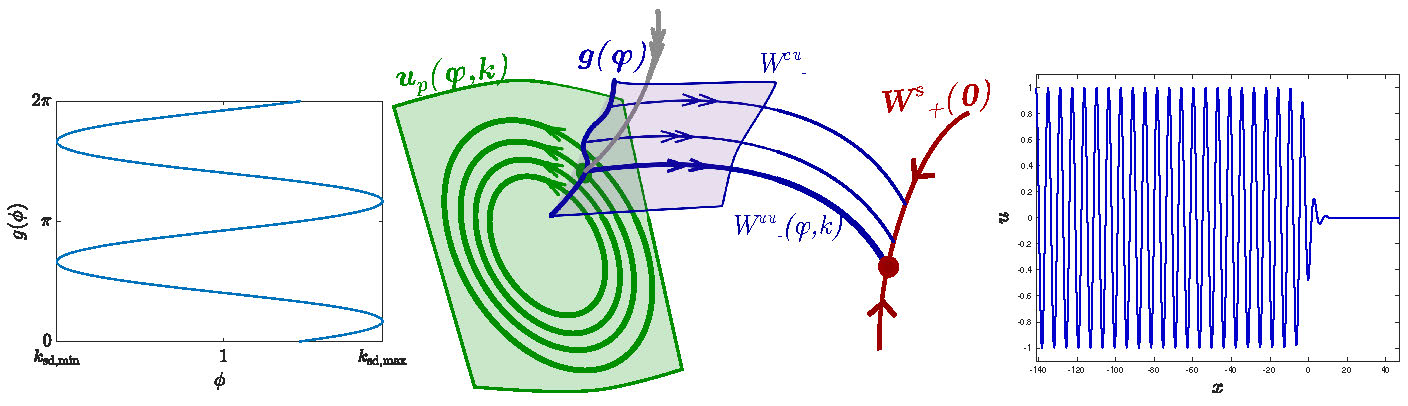
Figure 2.1: Left: strain-displacement relation (2.2) for \(\mu = 3/4\); Center: schematic phase-portrait of heteroclinic intersection in (2.1) (adapted with permission from [10, Figure 2(a)]; Copyrighted by the American Physical Society); Right: corresponding plot of the solution.

The works [32, 28] showed that the intersection can be parameterized in terms of the asymptotic phase \(\phi\) and wavenumber \(k_x\) of solutions \(|u(x) - u_p(k_x x+\phi;k)|\rightarrow0, \,\, x\rightarrow-\infty\) with \(k_x = g(\phi)\), written as a graph over \(\phi\) for some periodic function \(g\). As \(g\) relates how stretched the pattern is to its asymptotic phase shift, it is known as the strain-displacement relation. The work [32] uses normal form techniques to establish existence of patterned fronts in (2.1) for \(0<\mu\ll1\) and determines the leading order expansion

\( g(\phi)= 1+\frac{\mu}{16}\cos(2\phi)+ \mathcal{O}(|\mu|^{3/2}) \).

(2.2)

The range of \(g\), \(k_x\in(k_\mathrm{sd,min},k_\mathrm{sd,max}):= (\min g, \max g)\), gives the wavenumbers allowed for a stationary quench. We note that this range is a proper subset in the existence domain \((k_\mathrm{ex,-},k_\mathrm{ex,+})\); see Figure 1.1, right. In this sense we say that the quench selects patterns; see Figure 1.1. The concept of a strain-displacement relation was introduced in [28] which studied the effect of boundary conditions on patterns. Examples of strain-displacement relations were also calculated in [10] for other pattern-forming equations.

We briefly remark that the \(c_x = 0, k_y,k_x\neq0\) regime can also be studied using dynamical systems arguments [2]. Here the associated spatial dynamical system possesses a Hamiltonian structure as well as conserved quantity coming from the \(y\)-translation symmetry. Paired with an analysis of wavenumber energetics, one can use these to show that oblique stripes for any \(k_y\) must select wavenumbers which satisfy \(k_\mathrm{zz}^2 = k_{x}^2+k_y^2\), where \(k_\mathrm{zz}\) is the wavenumber bounding the zig-zag instability region so that stripes with \(k\) \(<\) \(k_\mathrm{zz}\) undergo wrinkling instabilities.

Another limit amenable to spatial dynamics treatment is the upper boundary in \(c_x\) of \(\mathcal{M}\) where patterns detach from the quench; see Figure 1.3, right plot. This boundary is given by the spreading speed, \(c_\mathrm{lin}\), at which pattern-forming fronts invade the unstable state \(u\equiv0\) in the homogeneous domain \(\rho\equiv \mu\). For the supercritical nonlinearity \(\mu u - u^3\), the spreading speed and stripe wavenumber \(k_\mathrm{lin}\) can be predicted using only the linear information about the unstable state. The resulting nonlinear invasion fronts are known as pulled fronts. See [41] for a broad overview and [18, 4] for a mathematical treatment. The work [13] studies parallel striped fronts for \(c_x\lesssim c_\mathrm{lin}\). Here (1.7) forms an ill-posed dynamical system in \(x\) in the phase space of \(y\)-periodic functions, and front solutions again correspond to heteroclinic orbits. One then uses a multiple scales analysis and center-manifold reduction for each phase portrait \(\rho\equiv \pm \mu\) to study dynamics of bounded solutions near the origin. Relevant invariant manifolds are transversely unfolded in the wavenumber \(k_x\), so that for each \(c_x\lesssim c_\mathrm{lin}\) there exists a \(k_x\) near \(k_\mathrm{lin}\) with a heteroclinic intersection. Thus, \(k_x\) is determined by the quench speed. See also [14] for analogous results using absolute spectrum in the complex Ginzburg Landau equation to derive the leading-order dependence of \(k_x\) for \(c_x\lesssim c_x\).

2.2. Functional analytic approach: \(k_y\gtrsim0, \,\, c_x,k_x>0\)

We discuss the functional analytic approach in the context of perturbing parallel grown fronts \(c_x>0,k_x>0, k_y =0\) to weakly oblique fronts \(c_x, k_x,k_y >0\). Here, difficulties arise in the corresponding spatial dynamics formulation due to the change in the domain of the linear operator in (1.7) as \(k_y\) perturbs from 0. The functional analytic approach allows one to side step this issue, continue solutions \(u(x,y;k_y)\) in a smooth fashion, and obtain a leading order prediction for the horizontal wavenumber

\( k_x(k_y) = k_{x,0} + b k_y^2 + \mathcal{O}(k_y^2) \),

(2.3)

for a fixed \(c_x>0\), and where \(b\) is constant determined by the parallel front \(u(x,y;0)\) and its derivatives. We outline the approach in the rest of the section and refer to [13] for more detail.

Consider the linearization of the nonlinear PDE (1.7) about a front solution with \((k_x,k_y) = (0,k_x^*)\) and \(c_x>0\),

\( \mathbb{L}:= -(1+\partial_x^2)^2 + c_x(\partial_x+k_x^*\partial_y) + \rho(x) - 3u_*(k_x x+ y;k_x^*)^2,\qquad\quad (x,y)\in \mathbb{R}\times\mathbb{T}, \qquad \mathbb{T} = \mathbb{R}/2\pi \).

(2.4)

Due to a quadratic tangency of the spectrum of the asymptotic periodic pattern \(u_p\) with wavenumber \(k_x\), this operator is not Fredholm when posed on \(L^2(\mathbb{R}\times\mathbb{T})\). To regain Fredholm properties of \(\mathbb{L}\) and apply a Lyapunov-Schmidt reduction, one poses the operator in an exponentially weighted function space \(L^2_\eta(\mathbb{R}\times \mathbb{T}):=\{ f\,:\, \mathrm{e}^{\eta|x|} f(x,y)\in L^2\}\). These spaces penalize or allow growth at \(|x| = \infty\) for \(\eta>0\) and \(\eta<0\) respectively, and somewhat standard techniques [31, 19] show that \(\mathbb{L}\) is Fredholm with index 0 for \(\eta<0\) and index -1 for \(\eta>0\). Since weighted spaces with \(\eta<0\) are not Banach algebras and hence will not play nicely with polynomial nonlinearities, we pose the operator on a space with \(\eta>0\), thus requiring perturbations of the front \(u_*\) to be exponentially localized and precluding perturbing the entire front solution at once.

To get around this difficulty, we use a core-farfield decomposition

\( u(x,y) = w(x,y)+\chi(x)u_p(k_x x + y;k),\quad k^2 = k_x^2 + k_y^2 \)

(2.5)

where \(\chi\) is a smooth monotonic step function, with \(\chi \equiv 1\) for \(x\leq -d\), and \(\chi \equiv0\) for \(x>-d+1\), and \(w\) an exponentially localized function which corrects the far-field pattern near the quench. This decomposition, when inserted into the nonlinear equation, allows one to separate out the far-field dynamics, which are controlled explicitly through the parameters \(k_x,k_y\), from the local dynamics near the quenching interface. Indeed, inserting this perturbation into (1.7) and using the fact that \(u_p\) solves the equation with \(\rho \equiv \mu\), one obtains

\( 0 = \mathcal{F}(w,k_x;k_y,c_x):= \mathcal{L}(k_x,k_y,c_x) w + [\mathcal{L},\chi]u_p + \mathcal{N}(w+\chi u_p(k)) - \chi \mathcal{N}(u_p) \),

(2.6)

\( \mathcal{L}(k_x,k_y,c_x) = -(1+\partial_x^2+k_y^2\partial_y^2)^2 + \rho + c_x(\partial_x + k_x\partial_y),\,\, \mathcal{N}(u) = -u^3,\qquad [\mathcal{L},\chi]v = \mathcal{L}(\chi v) - \chi\cdot \mathcal{L} v \).

(2.7)

One can show this operator is locally well-defined as a mapping on a suitable anisotropic Sobolev space with exponential weight, but is not smooth in \(k_y\) as a map near the parallel stripe solution \((w^*,k_x^*;0,c_x)\) where \(w_* = u_* - \chi u_p(k_x^*)\), since increased regularity in \(y\) is required for \(k_y\neq0\). This singular limit can be regularized using a bounded invertible operator \(\mathcal{P}(k_x,k_y,c_x):= (\mathcal{L}(k_x,k_y,c_x) - I)^{-1}\) to precondition the nonlinear operator, obtaining a new equation \(0 = \tilde{\mathcal{F}}:= \mathcal{P}\circ\mathcal{F}\) which is continuous with continuous derivatives in \(k_y\) near \(k_y = 0\). Under certain genericity assumptions on the parallel solution, one obtains that the new linearization \(\mathcal{P}(k_x,0)\circ\mathbb{L}\) is Fredholm with index -1 and one-dimensional cokernel (and thus trivial kernel), and \(\partial_{k_x} \tilde{\mathcal{F}}\Big|_{(w^*,k_x^*,0)}\not\in \mathrm{Rg} \mathcal{P}(k_x^*,0)\circ\mathbb{L}\). This implies the extended linearization \([\mathcal{P}\circ\mathbb{L},\mathcal{P}\circ\partial_{k_x}\mathcal{F}]\) is Fredholm index zero with trivial kernel. One can then apply the implicit function theorem to solve for \((w,k_x)\) in terms of \(k_y\), obtaining existence of oblique fronts as well as the leading order expansion for \(k_x(k_y)\).

2.3. Numerical continuation

We also mention that the functional analytic approach inspires a computational approach which represents heteroclinic profiles on a bounded computational domain. Here the far-field solution is formed by solving the 1-D roll equation (1.3) to find \(u_p(\theta;k)\) and then rotating the roll to obtain \(u_p(k_x x+y; k)\) for a given \(k_x,k_y\) pair. Being localized near the quench, one can approximate \(w\) on a bounded domain using periodic or Dirichlet boundary conditions. Appending a pseudo-arclength continuation algorithm, previous works have used this approach to continue quenched patterns [2], study pattern selection for a fixed boundary condition [28], grain-boundaries [22], and spiral waves [7]. Here one can discretize the spatial variables using any desired method. For example the work [2] used finite-differences in the \(x\)-direction, pseudo-spectral in the \(y\)-direction, and the built-in nonlinear solver in MATLAB. The work [3] paired a spectral Galerkin discretization in both \(x\) and \(y\) with a Newton-GMRES nonlinear solver to take advantage of spectral accuracy and GPU parallelization. See these references as well as [12] for more detail about this numerical approach.

2.4. Modulational techniques

Wavenumber selection and dynamics of grown patterns can also be understood using simplified equations which describe small amplitude and long wavelength modulations of periodic stripes. We discuss several examples which show how modulational approaches can be used to study slowly grown parallel and weakly oblique stripes, slowly grown accute oblique stripes, as well as perpendicular stripes.

2.4.1. Slowly grown parallel and oblique stripes: \(c_x,k_y\gtrsim0\)

One can study the dynamics of slowly grown parallel and oblique stripes using phase modulation equations. Here, phase perturbations of stable stripes \(u\sim \epsilon R(\epsilon x,\epsilon^2 t) \mathrm{e}^{\mathrm{i} \phi(\epsilon x,\epsilon^2 t)}\mathrm{e}^{\mathrm{i} x}+\mathrm{c.c.},\,\, \mu = \epsilon^2 \ll1\) can be described at leading order, after suitable scalings, by a linear diffusion equation \(\phi_t = d_\mathrm{eff}\Delta \phi\). Here \(\phi\) governs local phase dynamics of a perturbed periodic stripe, \(\nabla \phi\) gives local wavenumber modulations, and \(d_\mathrm{eff}\) gives the effective diffusivity of phase perturbations. To model the quench, we move to a horizontal co-moving frame, restrict to the left half-plane, and impose a nonlinear boundary condition determined by the strain displacement relation \(g\) defined above. In sum,

\( \phi_t = d_\mathrm{eff} \Delta \phi + c_x \phi_x,\qquad x<0, y\in \mathbb{R} \)

(2.8)

\( \phi_x = g(\phi),\qquad x = 0, y\in \mathbb{R} \).

(2.9)

In this equation, patterned front solutions with wavenumbers \((k_x,k_y)\) are represented by solutions \(\phi(x,k_y(y - c_yt))\) which are periodic in the co-rotating frame variable \(\tilde{y} = k_y y - k_y c_y t\) modulo \(2\pi\), \(\phi(x,\tilde{y}+2\pi/\omega) = \phi(x,\tilde{y})+2\pi\), and asymptotically linear \(|\phi(x,\tilde{y}) - (k_x x + \tilde{y})|\rightarrow0,x\rightarrow-\infty\). Here the temporal frequency \(\omega\) is 1:1 resonant with the horizontal far-field pattern \(\omega = c_x k_x\), and \(c_yk_y = c_xk_x\) relating the vertical and horizontal phase speed of stripes in the co-moving frame. Such a solution is depicted in Figure 2.2, and one can relate it to patterned solutions via \(\cos(\phi)\). In the slow growth regime, one observes a singularity at \(k_y = c_x = 0\), where the curves \(k_x(k_y,c_x)\) with fixed \(k_y>0\) converge setwise to the union of the vertical band \(\{(0,0,k_x)\,|\, k_x\in \mathrm{Rg }\, g\}\) and the monotontically increasing curve \(k_x(0,c_x)\) for parallel stripes which satisfies \(k_x(0,c_x)\rightarrow k_\mathrm{sd,min}\) as \(c_x\searrow 0\). In this region solutions develop a localized dislocation defect near the interface which mediates wavenumber selection in the bulk. For \(k_y = 0\), this kink corresponds to a slow stretching and fast snapping of the local phase in time near the boundary \(x = 0\).

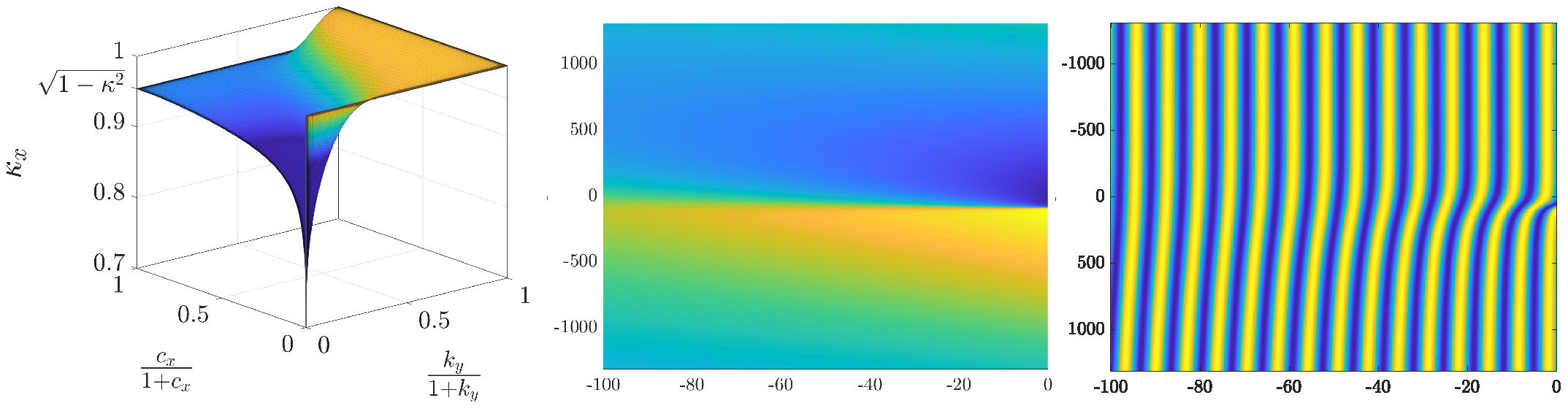
Figure 2.2: Left: Compactified plot of Moduli space for (2.8) (Reproduced from [3, Figure 1.2]); Center: Profile of \(\psi := \phi - (k_x x + k_y \tilde{y})\) in co-rotating frame for \(0\) \(<\) \(c_y,k_y\ll1\); Right: Plot of \(\cos(\phi(x,\tilde{y}))\).

We remark here that such a phase-diffusion approximation only describes parallel stripe formation in (1.7) when posed on a one-dimensional spatial domain as only then are all wavenumbers \(k\in (k_\mathrm{sd,min},k_\mathrm{sd,max})\) stable. In the two-dimensional isotropic equation (1.1) stripes with \(k\in(k_\mathrm{sd,min},k_\mathrm{zz})\) are zig-zag unstable and a different modulational approximation, such as the Cross-Newell equation, is required. The work [3] rigorously studies solutions of (2.8), derives wavenumber asymptotics, and accurately predicts solutions in a \(2\)D directionally quenched anisotropic Swift-Hohenberg equation, where the zig-zag instability is suppressed and all stripes \(k\in (k_\mathrm{sd,min},k_\mathrm{sd,max})\) are stable. In the one-dimensional case, see also [10] for formal asymptotic expansions and wavenumber predictions, and [29] for a rigorous analysis of (2.8) in \(1\)-D.

2.4.2. Slowly grown acute oblique stripes: \(c_x\gtrsim0, k_y\sim k_\mathrm{zz}\)

A modulational approach can also be used to study horizontal modulations of slowly grown perpendicular stripes with zig-zag critical wavenumber \(k_y\sim k_\mathrm{zz} = 1+\mathcal{O}(\mu^2)\) [2]. Once again neglecting the quench, \(\rho \equiv\mu\) and inserting the ansatz \(u(x,y,t) = \epsilon \mathrm{e}^{\mathrm{i} k_y y} R(\epsilon x,\epsilon t)\mathrm{e}^{\mathrm{i}\phi(\epsilon x,\epsilon t)} + \mathrm{c.c.}\) with \(k_y = 1 - \epsilon\). After scaling, and reducing to leading order, and taking one spatial derivative \(\psi = \nabla\phi\), one obtains a Cahn-Hilliard equation \(\psi_t = -(\psi_{xx} + \psi - \psi^3)_{xx}\). To model quenched patterns in this context, one moves into a co-moving frame and appends Dirichlet boundary conditions,

\( \psi_t = -(\psi_{xx} + \psi - \psi^3)_{xx}+c_x \psi_x,\,\,\, x<0 \qquad \psi = \psi_{xx}=0,\,\, x = 0 \).

(2.10)

Here oblique striped fronts correspond to equilibrium front solutions with \(\psi(x)\rightarrow \eta, x\rightarrow-\infty\) for some constant \(\eta\neq0\) which measure the asymptotic horizontal wavenumber.

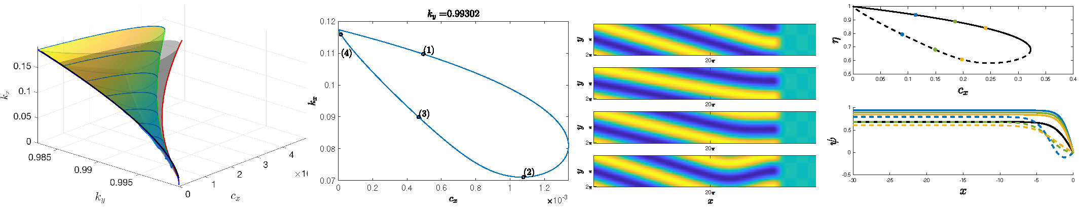
Figure 2.3: Left: Zoom in of the kink-dragging bubble in \(\mathcal{M}\) with \(\mu = 1/4\) along with the associated bubble from continuing fronts in (2.10) (grey); Center-left: cross section of bubble in \(\mathcal{M}\) for a fixed \(k_y\); Center-right: Solution profiles of (1.7) along this cross section; Right: Kink-dragging bubble bifurcation diagram in (2.10), comparing front asymptotic value \(\eta\) with front speed \(c_x\), solid line denotes stable solutions while dashed line gives unstable solutions, bottom inset gives example profiles \(\psi_*(x)\) for points along the stable (solid) and unstable (dashed) branches. First three plots reproduced from [2, Figures 16 and 20] while last plot uses data also from this work.

A functional analytic approach similar to that discussed above allows one to rigorously continue fronts in \(c_x\gtrsim0\). Numerical continuation then shows that such fronts undergo a saddle-node bifurcation at a speed \(c_\mathrm{x,osn}\). Passing through this point, the corresponding solution \(\psi(x)\) develops a kink in its profile; see Figure 2.3, right plot. In the original equation, such solutions are oblique stripes with an anti-phase kink, or "wrinkle" in the solution near the interface. Continuing such solution branches in \(k_y\) one observes an expanding "bubble", bounded by the fold curve \(c_\mathrm{x,osn}(k_y)\) which emanates from the point \((k_y,c_x,k_x) = (k_\mathrm{zz},0,0)\) in \(\mathcal{M}\). We mention that if one studies the time-dependent equation for speeds just above this fold, one observes a saddle-node on a limit-cycle where wrinkles in the striped phase are periodically shed in time, with growing period as \(c_x\) decreases to \(c_\mathrm{x,sn}\).

2.4.3. Perpendicular Stripes: \(k_x = 0\)

To model the perpendicular stripe regime of \(\mathcal{M}\), one can use an unscaled ansatz of the form \(u(x,y,t) = A(x,t) \mathrm{e}^{\mathrm{i} k_y y} + \mathrm{c.c.}\) in the full quenched equation (1.5) to obtain, at lowest order in powers of \(\mathrm{e}^{\mathrm{i} y}\), the Newell-Whitehead-Segel equation

\( A_t = -(1+\partial_x^2 - k_y^2)^2 A + \rho(x)A - 3A|A|^2 + c_x \partial_x A \).

(2.11)

When \(\rho\equiv \mu\), \(A_p\equiv \frac{\mu - (1-k_y^2)^2}{3}\), represents a perpendicular stripe and fronts \(A(x)\) connecting \(A_p\) with the trivial state \(A\equiv0\) represent perpendicular striped front solutions; see Figure 2.4, right plot, for a few examples. Numerically continuing fronts in parameters \(k_y\) and \(c_x\), one finds a broad domain of existence (plotted in Figure 2.4 left), bounded above by a curve \(c_\mathrm{x,psn}(k_y)\) of saddle-node points. Passing through this curve, the monotone front solution \(A(x)\) develops an anti-phase kink near the quench interface at \(x = 0\) in a manner similar to the acute oblique stripes discussed above. For speeds just below this bifurcation point we also find the perpendicular front undergoes a \(y\mapsto-y\) symmetry breaking pitchfork bifurcation at the points \(c_\mathrm{x,opf}(k_y)\). Here oblique stripes bifurcate and continue on to form the main "wing" of \(\mathcal{M}\). As \(k_y\) is decreased, the saddle-node curve \(c_\mathrm{x,psn}\) disappears in a cusp bifurcation. Near this bifurcation there are a wealth of different phenomena and solution branches, including collapsed snakes, isolas, and bifurcating oblique stripes which continue upwards in \(k_x\) and collide in a hyperbolic catastrophe with the oblique kink-forming bubble discussed in Section 2.4.2 above. See [2, Sections 5 and 6] for more detail.

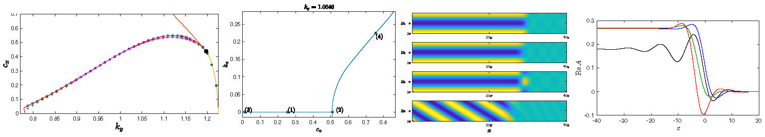
Figure 2.4: Left: Domain of existence of perpendicular stripes predicted by (2.11), bounded above by bifurcation curves \(c_\mathrm{x,psn}(k_y), c_\mathrm{x,opf}(k_y)\) (red and magenta), blue and green points indicate numerically measured bifurcation values in (1.7); Center Left: cross-section of \(\mathcal{M}\) with fixed \(k_y\) illustrating the perpendicular to oblique bifurcation; Center-Right: Solution profiles along this cross-section; Right: front solutions of (2.11) representing perpendicular stripes for various \(c_x,k_y\) values label in center-left plot; \(\mu = 1/4\) throughout, reproduced from [2, Figures 14, 17, and 19].

3. Outlook

There are many avenues to continue this line of study and we list a few below. In the directionally quenched Swift-Hohenberg equation, several regions are yet to be understood even on the heuristic level, including the location of the perpendicular stripe detachment saddle-node curve, the oblique stripe reattachment pitchfork bifurcation curve, as well as the weakly oblique, slowly growing stripe regime \(k_y,c_x\sim0\). It would also be of interest to apply analytic continuation and global bifurcating techniques to rigorously establish solutions in the bulk of the moduli space. Furthermore, there are several limits and boundaries of \(\mathcal{M}\) which are understood only from a heuristic, phenomenological, or modulational standpoint and still require a rigorous analysis.

Moving on from the existence analysis discussed here, one could also study stability of these pattern forming fronts. We refer to [2, Sections 4 and 5] for a discussion on zig-zag, cross-roll, and amplitude far-field instabilities of grown stripes and [11] for a rigorous study of spectral stability in a 1-D quenched complex Ginzburg Landau equation. In addition to stability, one could use modulational approximations as discussed in Section 2.4 to study dynamics and interactions of defect-laden patterns in the wake of the quench observed in Figure 1.3. As mentioned in the introduction, we also aim to characterize moduli spaces for different versions of the Swift-Hohenberg equation and in new models. The upcoming review paper [12] gives numerical results for an anisotropic version of (1.1) with an additional term \(\beta \partial_y^2 u\) (see also [3]) as well as a version of (1.1) with a subcritical quintic nonlinearity \(\rho(x)u+\gamma u^3 - u^5\). It also gives numerical continuations of the moduli space for a quenched 2-D complex Ginzburg Landau equation, as well as the two-species light-sensing CDIMA reaction-diffusion model.

There are of course many other systems in which one could study the moduli space for a directional quench-type heterogeneity. Examples include the Cahn-Hilliard or Allen-Cahn equations (see [27, 26] for results in this direction), phase-field systems, or various types of reaction-diffusion systems, such the Fitzhugh-Nagumo, Gierer-Meinhardt, or Klausmeier equations. One could also move away from directional quenching and consider patterns for different quenching geometries \(\Omega_t\) as depicted in Figure 1.2. Along these lines, it would be interesting to relate our area of study to recent works which study phenomenology of Turing patterns in evolving domains in the context of morphogenesis and reaction-diffusion models; see [21] for a recent review.

Even further, there are many other types of heterogeneities of applicational interest, including slow ramps, localized functions, and periodically modulated functions. Mathematically, these applied problems give a rich playground for the application, combination, and further development of tools from applied PDE, dynamics, numerics, and beyond.

Acknowledgment

This work was partially supported through NSF-DMS 2006887.

References

[1]   S. Akamatsu, S. Bottin-Rousseau, and G. Faivre, Experimental evidence for a zigzag bifurcation in bulk lamellar eutectic growth, Phys. Rev. Lett., 93 (2004), p. 175701.

[2]   M. Avery, R. Goh, O. Goodloe, A. Milewski, and A. Scheel, Growing stripes, with and without wrinkles, SIAM Journal on Applied Dynamical Systems, 18 (2019), pp. 1078-1117.

[3]   K. Chen, Z. Deiman, R. Goh, S. Jankovic, and A. Scheel, Strain and defects in oblique stripe growth, arXiv preprint arXiv:2102.02905, 2021.

[4]   P. Collet and J.-P. Eckmann, Instabilities and fronts in extended systems, Princeton University Press, 2014.

[5]   E. Crampin, W. Hackborn, and P. Maini, Pattern formation in reaction-diffusion models with nonuniform domain growth, Bulletin of mathematical biology, 64 (2002), pp. 747-769.

[6]   J. H. Dawes, After 1952: The later development of Alan Turing's ideas on the mathematics of pattern formation, Historia Mathematica, 43 (2016), pp. 49-64.

[7]   S. Dodson and B. Sandstede, Determining the source of period-doubling instabilities in spiral waves, SIAM Journal on Applied Dynamical Systems, 18 (2019), pp. 2202-2226.

[8]   E. M. Foard and A. J. Wagner, Survey of morphologies formed in the wake of an enslaved phase-separation front in two dimensions, Phys. Rev. E, 85 (2012), p. 011501.

[9]   R. Friedrich, G. Radons, T. Ditzinger, and A. Henning, Ripple formation through an interface instability from moving growth and erosion sources, Phys. Rev. Lett., 85 (2000), pp. 4884-4887.

[10]   R. Goh, R. Beekie, D. Matthias, J. Nunley, and A. Scheel, Universal wave-number selection laws in apical growth, Phys. Rev. E, 94 (2016), p. 022219.

[11]   R. Goh and B. de Rijk, Spectral stability of pattern-forming fronts in the complex ginzburg-landau equation with a quenching mechanism, arXiv preprint arXiv:2006.15083, 2020.

[12]   R. Goh and A. Scheel, Quenched stripes, In preparation.

[13]   R. Goh and A. Scheel, Pattern-forming fronts in a Swift-Hohenberg equation with directional quenching - parallel and oblique stripes, Journal of the London Mathematical Society, 98 (1999), pp. 104-128.

[14]   R. Goh and A. Scheel, Triggered fronts in the complex Ginzburg Landau equation, J. Nonlinear Sci., 24 (2014), pp. 117-144.

[15]   R. Goh and A. Scheel, Hopf bifurcation from fronts in the Cahn-Hilliard equation, Archive for Rational Mechanics and Analysis, 217 (2015), pp. 1219-1263.

[16]   M. Haragus and G. Iooss, Local bifurcations, center manifolds, and normal forms in infinite-dimensional dynamical systems, Springer Science & Business Media, 2010.

[17]   T. Hiscock and S. Megason, Orientation of Turing-like patterns by morphogen gradients and tissue anisotropies, Cell Systems, 1 (2015), pp. 408-416.

[18]   M. Holzer and A. Scheel, Criteria for pointwise growth and their role in invasion processes, J. Nonlinear Sci., 24 (2014), pp. 661-709.

[19]   T. Kapitula and K. Promislow, Spectral and dynamical stability of nonlinear waves, Springer, 2013.

[20]   C. Konow, N. H. Somberg, J. Chavez, I. R. Epstein, and M. Dolnik, Turing patterns on radially growing domains: experiments and simulations, Physical Chemistry Chemical Physics, 21 (2019), pp. 6718-6724.

[21]   A. L. Krause, E. A. Gaffney, P. K. Maini, and V. Klika, Modern perspectives on near-equilibrium analysis of turing systems, arXiv preprint arXiv:2106.08375, 2021.

[22]   D. J. B. Lloyd and A. Scheel, Continuation and bifurcation of grain boundaries in the Swift-Hohenberg equation, SIAM J. Appl. Dyn. Syst., 16 (2017), pp. 252-293.

[23]   A. Mielke, Instability and stability of rolls in the Swift-Hohenberg equation, Communications in Mathematical Physics, 189 (1997), pp. 829-853.

[24]   D. G. Míguez, M. Dolnik, A. P. Munuzuri, and L. Kramer, Effect of axial growth on turing pattern formation, Physical review letters, 96 (2006), p. 048304.

[25]   S. A. Mollick, D. Ghose, P. D. Shipman, and R. Mark Bradley, Anomalous patterns and nearly defect-free ripples produced by bombarding silicon and germanium with a beam of gold ions, Applied Physics Letters, 104 (2014), p. 043103.

[26]   R. Monteiro, Horizontal patterns from finite speed directional quenching, Discrete & Continuous Dynamical Systems-B, 23 (2018), p. 3503.

[27]   R. Monteiro and A. Scheel, Phase separation patterns from directional quenching, Journal of Nonlinear Science, 27 (2017), pp. 1339-1378.

[28]   D. Morrissey and A. Scheel, Characterizing the effect of boundary conditions on striped phases, SIAM Journal on Applied Dynamical Systems, 14 (2015), pp. 1387-1417.

[29]   A. Pauthier and A. Scheel, Advection-diffusion dynamics with nonlinear boundary flux as a model for crystal growth, Math. Nachr., 293 (2020), pp. 1565-1590.

[30]   M. F. Pennybacker, P. D. Shipman, and A. C. Newell, Phyllotaxis: Some progress, but a story far from over, Physica D: Nonlinear Phenomena, 306 (2015), pp. 48-81.

[31]   B. Sandstede and A. Scheel, Relative Morse indices, Fredholm indices, and group velocities, Discrete Contin. Dyn. Syst., 20 (2008), pp. 139-158.

[32]   A. Scheel and J. Weinburd, Wavenumber selection via spatial parameter jump, Philos. Trans. Roy. Soc. A, 376 (2018), pp. 20170191, 20.

[33]   G. Schneider, Diffusive stability of spatial periodic solutions of the Swift-Hohenberg equation, Communications in mathematical physics, 178 (1996), pp. 679-702.

[34]   R. Sheth, L. Marcon, M. F. Bastida, M. Junco, L. Quintana, R. Dahn, M. Kmita, J. Sharpe, and M. A. Ros, Hox genes regulate digit patterning by controlling the wavelength of a Turing-type mechanism, Science, 338 (2012), pp. 1476-1480.

[35]   N. Stoop and J. Dunkel, Defect formation dynamics in curved elastic surface crystals, Soft Matter, 14 (2018), pp. 2329-2338.

[36]   J. Swift and P. C. Hohenberg, Hydrodynamic fluctuations at the convective instability, Phys. Rev. A, 15 (1977), pp. 319-328.

[37]   U. Thiele, Patterned deposition at moving contact lines, Advances in Colloid and Interface Science, 206 (2014), pp. 399-413. Manuel G. Velarde.

[38]   S. Thomas, I. Lagzi, F. Molnár, and Z. Rácz, Helices in the wake of precipitation fronts, Phys. Rev. E, 88 (2013), p. 022141.

[39]   T. Tsukada and R. Kurita, A topological transition by confinement of a phase separating system with radial quenching, Scientific reports, 9 (2019), pp. 1-10.

[40]   A. M. Turing, The chemical basis of morphogenesis, Philosophical Transactions of the Royal Society of London. Series B, Biological Sciences, 237 (1952), pp. 37-72.

[41]   W. van Saarloos, Front propagation into unstable states, Physics Reports, 386 (2003), pp. 29-222.

[42]   M. Wilczek, W. B. H. Tewes, S. V. Gurevich, M. H. Köpf, L. F. Chi, and U. Thiele, Modelling pattern formation in dip-coating experiments, Math. Model. Nat. Phenom., 10 (2015), pp. 44-60.