Handling editor: Evelyn Sander

The Dynamics of Toys

G. Bard Ermentrout, Department of Mathematics and University Professor of Computational Biology, University of Pittsburgh
and John G. Milton, William R. Kenan Jr. Professor of Computational Neuroscience and Department of Biology, The Claremont Colleges

The ability of toys and play to awaken mathematical curiosity stems from their interesting motions, which range from periodic oscillations to even chaos. Since these movements are governed by the toy's intrinsic physical properties it is relatively easy to generate models in the form of differential equations. However, can these models capture the observed dynamics? The increasing availability of inexpensive, easy-to-use motion capture technologies makes it possible to quantitatively compare model to toy. These approaches identify a number of unresolved mathematical problems whose solutions may ultimately provide insights into why the nervous system is so fascinated with toys and play.

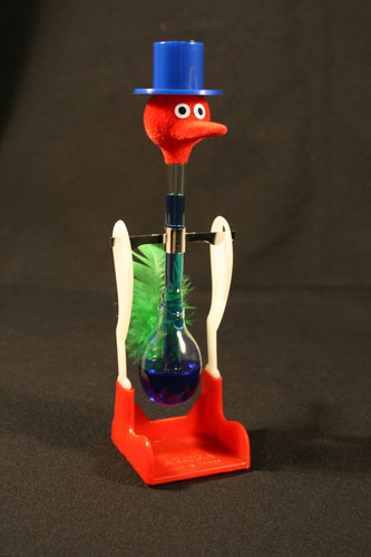
(Fig. A) The drinking bird.

(Movie B) Movie of drinking bird.

Drinking bird

A large family of toys exploits gravity and the swinging motion of pendulums. Indeed many carnival rides and "chaotic" toys are periodically driven damped pendulums. However, by far the most famous pendulum toy is the drinking bird (Fig. A). The drinking bird's résumé includes starring roles in cartoons and movies and it functions as the unofficial mascot for a well-known scientific equipment supplier.

The characteristic "drinking movements" (Movie B) are the result of a dynamic heat engine that exploits liquid-vapor equilibrium in order to convert heat energy into a pressure differential within the device, and hence perform mechanical work. Evaporative cooling lowers pressure and causes fluid to rise into the bird's head. Once the mass of the bird's head becomes sufficiently heavy the head drops and is wetted, the pressure seal is broken so that fluid returns to the base and the head is raised again.

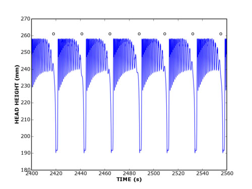
(Fig. C) Time series showing cycle-to-cycle variation in drinking bird wave-forms. This graph was obtained by experimental observation of a drinking bird with a reflective marker on its head.

Up until now the scientific investigations have focused on determining the thermodynamic efficiency of the bird heat engine and probing the effects of temperature differentials and humidity on the period of the bird's dunking motions [1-3]. However, to see the richness of the range of dynamics of the bird we put a reflective marker on its head and recorded its movements. Look closely at the right shoulder of the oscillation dunking cycle (Fig. C) (indicated by an 'o' above the graph). The waveform morphology is not constant but instead varies from cycle to cycle. Moreover, it clearly depends on what the bird is drinking (Fig. CC).

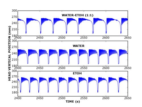
(Fig. CC) A time series recording from a drinking bird using three different types of fluids. This graph was obtained experimentally using the same methods as used in Fig. C.

What does mathematics say about the drinking bird? Well, the differential equations that describe the motions of the drinking bird can be readily obtained from a mechanical model (Fig. D) using the Euler-Lagrange formulation

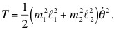
where the Lagrangian, L, is equal to the difference between the kinetic energy (T) and potential energy (U), L= T - U,

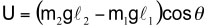
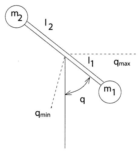
(Fig. D) A mechanical picture of the bird toy model.

Here the total mass is M=m₁+m₂, and the reset condition is that when θ hits a critical value, m₂ is reset and the velocity is set to zero. In order to complete the model it is necessary to account for the effects of evaporative cooling. The simple assumption that evaporative cooling causes the mass of the bird's head to increase proportional to swinging speed, i.e. , yields the predictions of this model (Fig. E). Although there is remarkable similarity between the predicted and observed motions of the bird there is one important discrepancy. Namely, variation in the waveforms are observed experimentally, but they are not predicted by the model. Certainly the addition of noise to the model causes the waveforms to vary, but what is the source of the noise? Maybe the bird model requires us to be more creative about the description of the evaporative cooling of the bird's head or perhaps the reset condition is too naïve. Certainly, there are small eddies created by the motion of the bird and this could provide a source of "noise" in the evaporation rate. More obviously, look at the movie of the bird as it hits its base. It does not come to a complete stop, but, rather, bounces a few times before rocking back. How could this be modeled? What's your idea? This is where the fun begins.

(Fig. E) Numerical simulation of the bird model with and without a small amount of randomness (noise).

Stick balancing

It is one thing to watch a toy in action, yet another to play with it. Just invert the pendulum and we have a toy that most of us have played with at one time or the other, namely, stick balancing at the fingertip (Movie F). The fact that longer sticks are easier to balance than shorter ones arises because it takes time for the nervous system to detect the vertical displacement angle and make a correction: once the stick becomes sufficiently long its rate of movement becomes slow compared to the correction time and hence balancing becomes easier. Thus a reasonable model for stick balancing is the delay differential equation of the form

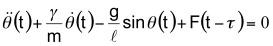
where θ is the vertical displacement angle (θ=0 corresponds to the upright position, hence the "-" sign), τ is the neural latency, k is the damping coefficient, and g is the gravitational constant. Intuitively the feedback, F, is negative, i.e. when θ increases, F acts in a manner to decrease iwt. Mathematical analysis of this equation suggests that the upright position is stable provided that the neural time delay, τ_n, is shorter than a critical time delay, τ_c, proportional to . In other words, for sufficiently long sticks the upright position of the stick balanced at the fingertip is stable.

(Movie F) This movie shows an example stick balancing on the fingertip.

Play at stick balancing for just a few minutes and you can readily see that these expectations are not true. For example, even long sticks fall. In addition, high speed motion capture in three dimensions suggest that the feedback is positive, not negative and moreover that the feedback corrections do not occur continuously but in an intermittent, or "ballistic" manner [4]. More surprising is the fact that more than 95% of the time intervals between successive corrective movements are shorter than the neural latency. These observations highlight the complexity of control in the presence of feedback delay and noise. In particular, how are those fluctuations that need to be acted upon by the controller distinguished from those that do not? This is because, by definition, there is a finite probability that an initial deviation away from a set point will be counter--balanced by one towards the set point just by chance. Too quick a response by a controller to a given deviation can lead to the phenomenon of "over control" leading to destabilization, particularly when time delays are appreciable. On the other hand, waiting too long runs the risk that the control may be applied too late to be effective. Thus methods based on continuous feedback control are not only anticipated to very difficult to implement by the nervous system, but also are unlikely to be effective. As a consequence mathematical attention is drawn to issues such as control at the "edge of stability" and the importance of "act and wait" control strategies [5,6]. In other words without the benefit of motion capture techniques a mathematician could easily have missed the important range of problems associated with stick balancing at the fingertip.

(Movie G) This movie shows stick balancing with and without leg shaking.

Most applied mathematicians do not have the opportunity to actively participate in the scientific method of making quantitative comparisons between theory and prediction. With the ready availability of motion capture technologies studies of the dynamics of toys present unique opportunities to study dynamical systems. The driving force is the fact that discrepancies between existing toy models and observed dynamics exist. These discrepancies provide an opportunity to learn about how complex dynamics of the toy are impacted by noisy perturbations and the controlling strategies of the nervous system that plays with the toy. In 2009 there will be a 5-day workshop at the Banff International Research Station (BIRS, Nov. 8-13, 2009) on the time-delayed control of noisy inverted pendulums that uses toys and on-site motion capture equipment to enable scientists to exchange ideas in a setting that promotes "mathematicans and science in action." Since physical properties determine the dynamics of toys, laboratory experiences can be designed so that differential equations can be readily learned by students "hands on." Thus as your children tire of the toys they received over the holiday season, it might be worthwhile to pick them up and play with them. Hmmm... interesting mathematics? More importantly it's actually fun (Movie G).

Acknowledgements

Special thanks to R. Fraiser, J. Gyorffy, D. Jaurequi, R. Knox and T. Ohira.

References

[1]		Güémez J, Valiente R, Fiolhais C and Fiolhais M (2003). Experiments with the drinking bird. Am. J. Phys. 71: 1257-1263.
[2]		Lorenz, R (2006). Finite-time thermodynamics of an instrumented drinking bird toy. Am. J. Phys. 74: 677-682.
[3]		Ng LM and Ng YS (1993). The thermodynamics of the drinking bird toy. Phys. Educ. 28: 320-324.
[4]		Cabrera JL and Milton JG (2002). On-off intermittency in a human balancing task. Phys. Rev. Lett. 89: 158702
[5]		Milton JG, Cabrera JL and Ohira T (2008). Unstable dynamical systems: Delays, noise and control. Europhysics Lett. 83: 48001.
[6]		Insperger T (2006). Act-and-wait concept for continuous-time control system with feedback delay. IEEE Trans. Control Sys. Tech. 14: 974-977.