I find most plenary talks at SIAM conferences to be rather spellbinding, but one is especially burned into my brain: Robert Ghrist’s Network Topology, Sensors and Systems, delivered at Snowbird in 2009. This talk was my first introduction to the idea that a set of discrete points could have a hole in it, a notion which blew my mind.

The Struggle

I graduated from college in 1996, 13 years before Ghrist’s talk. As an undergraduate, I majored in applied mathematics, taking calculus, linear algebra, differential equations, C programming, numerical analysis, applied complex variables, Fourier methods, basic probability and statistics, and a smattering of other topics. My program did not require any real analysis, abstract algebra, or topology, and I didn’t manage to brush against these subjects until later in my academic career. I learned some abstract algebra as a graduate student, when I used equivariant bifurcation theory to study fluid wave patterns. I learned some analysis as a postdoc, when I began working on continuum models of biological aggregations. Topology didn’t pop into my mathematical life – at least, not in an explicit way – until I was already an assistant professor.

At that Snowbird conference in 2009, Ghrist explored questions pertaining to sensor networks, one of which I’ll state in my own words here. Imagine you have to monitor some characteristic of the environment, say, temperature, pressure, or some other variable. To accomplish this task, you are given a large number of wireless sensors, each of which has a fixed, limited sensing range. The sensors might even move around over time. Because of the limitations of the hardware, it is difficult to know the exact location of the sensors at each moment, though the sensors are able to record which other sensors, if any, are within their sensing range. Given these constraints and capabilities, you’d like to know if there is a hole in your sensor network, which would correspond to an undesirable, un-sensed region. What’s a good way to do this?

In a style inspired by this this classic clip, the one-word answer to the problem is: topology. Well, that’s a bit glib. But as Ghrist eloquently explained, tools from algebraic topology do provide a great deal of insight. In 2009, while I didn’t understand all of the math in Ghrist’s talk, I nonetheless thought “this is really cool, and I should learn it!” But, busy with other projects, I did nothing about it for five years.

Then, things changed. In my research, I was faced with the challenge of how to grapple with large data sets. More specifically, I had long been interested in biological aggregations, that is, groups such as bird flocks, fish schools, and insect swarms in which individuals may interact socially and form emergent, coherent structures. Biological experiments on aggregations and numerical simulations of aggregation models each can give rise to a high volume of information.

Classic example of a biological aggregation: A flock of red-billed quelea comprising thousands of individuals. [https://en.wikipedia.org/wiki/Flock_(birds)#/media/File:Red-billed_quelea_flocking_at_waterhole.jpg]

As merely one example, consider a seminal model of Vicsek and collaborators (also reviewed here) in which point particles assume the average direction of travel of other particles that are sufficiently close. The model can produce various qualitatively different aggregate behaviors. What’s a good way to assess the state of the system, which might be characterized by the positions and headings of hundreds or thousands of particles? One of the classic ways to quantify the group dynamics has been to track the time evolution of an “order parameter” that measures the overall polarization of the group, that is, the extent to which the particles’ headings align with each other. When this order parameter is zero, particles are globally not aligned; when it is one, all particles are traveling in the same direction.  Other studies of aggregations have augmented this approach with other order parameters. For instance, this one looked at angular momentum, used to assess whether a group displays rotational motion.

These order parameters yield insight into group dynamics, but it seemed to me that to invoke them, you’d need to have an a priori instinct for the dynamics you wanted to detect. I wanted a way to quantify group dynamics without having to decide in advance what I was looking for (and we all know how it turns out when you are looking for something too specific).

 

The Triumph

Fortuitously, I had a new colleague in my department at Macalester College: Lori Ziegelmeier, who has experience in the field of topological data analysis. When I described my problem to Lori, she suggested that a technique called computational persistent homology – which I’ll explain at length below – might be a productive lens through which to view group dynamics. Then she sat down and tried to teach me some topology. Lori taught me brilliantly, and I’m going to tell you my version of what I learned from her. Lori understands all the mathematical underpinnings, including Morse functions, filtrations and other wonderful mathematical ideas. I don’t, so I am going to give you a heuristic explanation that will greatly scandalize you if you are an actual topologist.

Say you have a bunch of points. Fancy people call this a “point cloud of data.” I just call it a bunch of points. These points can live in almost any kind of space, but let’s just imagine for now that our space is Rⁿ. In the case of the biological aggregations, say that at one moment in time you had the three-dimensional positions and velocities of 5000 birds. You’d then have 5000 points in a six-dimensional space.

You don’t really know what you want to say about this data, so you decide that topology is a fairly agnostic way to analyze it. The way we’re going to do this is by measuring how many holes of various dimensions are in the data set. Knowing the number of holes of various dimensions doesn’t tell you everything, but it tells you a lot.

But wait, you say. How can a bunch of discrete points have a hole in them? The answer is that we’re going to imagine that our discrete points actually represent some object that is a bit less discrete. We’ll do that by taking our points and using them to build a simplicial complex. A simplicial complex is just a set of points, line segments, triangles, tetrahedrons, and so on up through higher dimensions. There are many ways to construct a simplicial complex from a set of points, but for our example, we’ll use the Vietoris–Rips complex. Here’s how it works. You pick an (arbitrary) connection distance. Call it ε. If two points are within ε of each other, connect them by a line segment. If three points are all pairwise within ε of each other, fill in the triangle that they form. If four points are all pairwise within ε of each other, fill in the tetrahedron that they form. Note here that you are potentially imposing a higher-dimensional structure on the data. For instance, if your data lives in two dimensions on a piece of notebook paper, and if you have four points that are all pairwise connected, you’d use your best artistic skills, including some shading, to draw a tetrahedron on your page, even though the points are co-planar. 

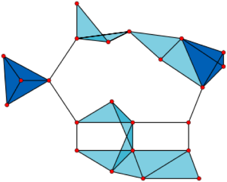
A Vietoris–Rips complex made up of 23 points in the plane. [https://en.wikipedia.org/wiki/Vietoris–Rips_complex#/media/File:VR_complex.svg]

Now that you’ve built an object out of your discrete set of points, you need homology, which helps you count the number of holes of various dimensions in that object . The quantities that count these holes are called Betti numbers (technically, each Betti number is the rank of a homology group, or so I am told). The quantity β₀ is the zeroth Betti number, which counts the number of holes of zero dimensions. It turns out that a “hole of zero dimensions” is just the complement of a connected component. So if your simplicial complex is made of three disconnected parts, you’d find β₀ = 3.  The first Betti number, β₁, counts the number of holes with a one-dimensional boundary, that is, topological circles (loops). The second Betti number, β₂, counts the number of holes with two-dimensional boundaries, that is, trapped volumes, and so on up through higher dimensions.

How should we count these holes? One way to do this is just by looking. But if you have a lot of data points and/or your data lives in a higher dimensional space that you can visualize, looking won’t be a feasible strategy. Algebraic topology provides a way to take the simplicial complex, encode it, and use mathematical machinery — essentially linear algebra — to calculate the number of holes. It’s a little beyond explaining in a brief, whimsical web article, but it can be explained in a slightly longer and substantially more whimsical tutorial. Fortunately, I have written one (which even features an appearance by international drag superstar RuPaul), Chad’s Self-Help Homology Tutorial for the Simple(x)-Minded (and here is a version that contains the answers to the exercises). This tutorial is written for people like me, who know no topology, but who are comfortable with basic linear algebra.

So far, all of this amounts to calculating homology. But what is persistent homology?

Recall that above, when building our simplicial complex, we chose an arbitrary distance ε over which to create connections between our data points. The main point of persistent homology is just to say heck, ε is arbitrary, so the best thing to do is to vary ε and calculate the homology over and over and over. What you get from doing this is that the Betti numbers are now functions of ε. Some topological features might be very short-lived. For instance, perhaps at extremely small values of ε there are lots of individual connected components, but many of them merge at slightly larger values. We might not be so interested in these transient (in scale) features, and would be tempted to interpret them as topological noise (though this is not always the case). However, topological features that exist over large ranges of ε are interpreted as being persistent, and hence more substantive features of the data. You might now want to ask how large a range of ε counts as large. It boils down to being contextual (and a bit arbitrary), and perhaps to being a matter suitable for statistical analysis.

There are several different ways to visualize the results of persistent homology calculations. One way is to use a horizontal axis representing ε and plot a stack of horizontal bars running between the ε values at which various topological features are born and die. These visualizations are called topological barcodes.

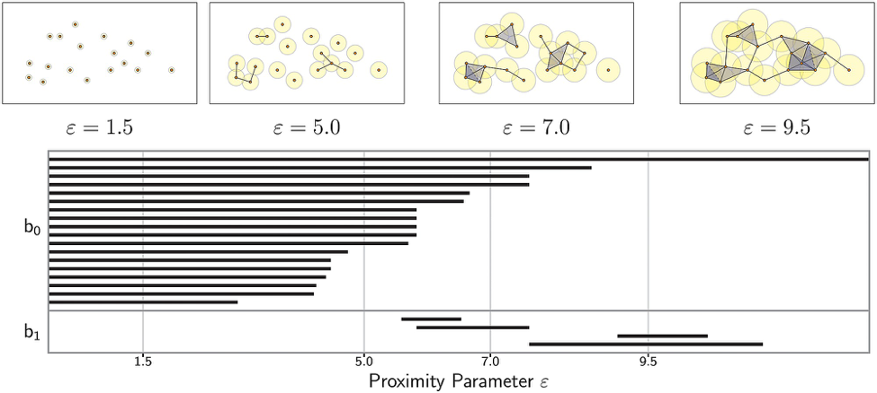
Topological barcode of the zeroth and first Betti numbers for 18 points in the plane. To infer the Betti number at a given scale ε, simply count the number of bars that exist for that value of ε. Top panels visualize the simplicial complex for four sample values of ε, each indicated by the radius of the balls around the data points. [http://journals.plos.org/plosone/article?id=10.1371/journal.pone.0126383]

It’s not too onerous to understand the idea of calculating homology (again, see my tutorial if you are interested). I highly recommend working out an example or two by hand. However, if you are going to calculate persistent homology on large data sets, you’ll need a computer, and indeed, this is the computational part of computational persistent homology. There are two steps in the computational process. First, you have to create a simplicial complex out of the data points. This is a problem in computational geometry. Second, you have to calculate homology. This is the algebraic topology part. Fortunately, many excellent computer packages exist to do the heavy lifting for you, including JavaPlex (which works with MATLAB), Dionysus, Perseus, and others.

There are now several classic books and papers on persistent homology and computational persistent homology, including work by: Kaczynski, Mischaikow, and Mrozek; Zomorodian and Carlsson; Ghrist; Edelsbrunner and Harer; and Carlsson. Additionally, you can find resources in a great Quora response thread started by the incomparable Mason Porter (the man, not the band). Finally, this overview paper is an invaluable resource, providing a review of the mathematical foundations of persistent homology as well as an introduction to various computational packages.

In the end, Lori and I and our colleague Tom Halverson used computational persistent homology to make sense of the data-hefty output of two biological aggregation models. Rather than manually looking at many individual frames of long numerical simulations to try to find interesting dynamical events and collective behavior, we examined how the kth Betti number varied over ε and over time, t. We call the visualization of β_k(ε,t) a Contour Realization Of Computed k-Dimensional hole Evolution in the Rips Complex, or for short, a CROCKER plot (get it?). We took note of topological transitions and of topological features that persisted over large scales and long times, and used the topological information to guide us in further exploration of the large data set.

 

The Struggle, Again

Topological data analysis (TDA) refers to a family of techniques and viewpoints aimed at looking at the shape of data. Arguably, computational persistent homology is the workhorse of TDA. TDA has been used to identify subtypes of breast cancer, study contagion on networks, analyze nursery rhymes, and much more.

As an applied mathematician whose career has, over the years, drifted towards data-intensive problems, I’ve found learning and using TDA to be irresistibly fun and scientifically rewarding. My new struggle is to continue learning enough topology to adapt TDA techniques to problems I see coming down the road in my research life. I hope I have convinced you, however, that with some linear algebra, a modest computer, and a little bit of moxy, you can start making use of tools from TDA.

 

Thanks to Tom Halverson, Mason Porter, and Lori Ziegelmeier for helpful feedback on this article.