Maxime Breden, CMAP, École Polytechnique, route de Saclay, 91120 Palaiseau, France ([email protected]).
Christian Kuehn, Technical University of Munich, Department of Mathematics, Research Unit "Multiscale and Stochastic Dynamics", 85748 Garching b. München, Germany ([email protected]).
Kerstin Lux, Technical University of Munich, Department of Mathematics, Research Unit "Multiscale and Stochastic Dynamics", 85748 Garching b. München, Germany ([email protected]).

1. Introduction

Climate change and pandemic dynamics are just a few of the pressing complex systems challenges that society is concerned with. Any mathematical model for a complex system is necessarily a reduced picture of reality. Yet, nonlinear dynamics models, e.g., involving differential equations, have proven incredibly helpful to understand typical effects and phenomena. To bridge reduction to realism, a common path is via stochastics. The idea is to encode extrinsic and intrinsic degrees of freedom using uncertain parameters or even include a stochastic process forcing the differential equation. There has been a long history trying to tackle the latter case focusing on stochastic ordinary and stochastic partial differential equations (SODEs/SPDEs). In this context, major technical complications arise as one deals effectively with non-autonomous dynamical systems, which also require tools from stochastic analysis. If the stochasticity is static in time, i.e., if one considers random ordinary or partial differential equations (RODEs/RPDEs) with uncertain parameters, technical complications seem to be reduced. After all, once parameters are sampled, one deals with a classical autonomous ODE/PDE. A focus has been put historically on the inverse problem of estimating parameter distributions from data, which is well-studied within the community of uncertainty quantification (UQ). Due to this history, one has almost completely overlooked the problem of pairing nonlinear dynamics with forward UQ, which itself poses several serious challenges as discussed below. More precisely, it is crucial for applications to study, what happens when we feed through nonlinear science concepts a parameter probability distribution. Here we provide an exposition to an entire research program currently in progress to develop new methods for nonlinear dynamics of RODEs/RPDEs. For exposition, we restrict to RODEs of the form

\( \frac{\mbox{d}x}{\mbox{d}t} = x' = f(x,p,q) \)

(1.1)

where \(x=x(t)\in\mathbb{R}^d\) is the unknown, \(p=p(\omega)\in\mathbb{R}^M\) are random parameters defined on a probability space \((\Omega,\mathcal{F},\mathbb{P})\), \(q\in\mathbb{R}^N\) are deterministic/control parameters, and \(f:\mathbb{R}^{d+N+M}\rightarrow \mathbb{R}^d\) is a sufficiently smooth vector field. If we sample \(p(\omega)\), then for each fixed \((p,q)\), standard existence and uniqueness ODE theory applies to (1.1). Hence, one is misled to believe that the standard tools from nonlinear dynamics carry over such as stability analysis, bifurcation theory, invariant manifolds and related techniques. Yet, this is only very partially correct. In fact, all objects we are accustomed to also become random. To actually make applicable conclusions, it is a natural task to analyze these objects from a probabilistic viewpoint. To illustrate this concretely, consider the following objects:

(R0)  random equilibria \(x^*(\omega,q)\) satisfying \(f(x^*(\omega),p(\omega),q)=0\),

(R1)  random periodic orbits \(\gamma(t,\omega,q)=\gamma(t+T(\omega,q),\omega,q)\),

(R2)  random stable/unstable eigenspaces and random stable/unstable manifolds,

(R3)  random bifurcation coefficients \(c(\omega,q)\), e.g., Lyapunov coefficients,

(R4)  random bifurcation diagrams.

It is often reasonable to assume that at some level, we deterministically have some information. For example, it sometimes makes sense to assume for (R0) that certain equilibrium branches are deterministic and well-understood; as concrete examples, think of the state of no infected individuals in epidemics or the state of a fluid at rest. Yet, most differential equations from applications will have dynamical objects that become random sets, when there are random input parameters present. The challenges we have to address are quite broad. One may ask, how to quantify the uncertainty of an object? Can we determine a suitable probability distribution associated to it? Is the computation possible analytically, or only numerically? If so, what are efficient algorithms? How to visualize the results? How to utilize the results in applications, e.g., how to quantify risk in nonlinear systems? Developing a toolbox to answer these questions is a program for several decades of research but recently several steps have been made, which we outline here. A main example we are going to use is a RODE version of the Lorenz equations

\( \left\{ \begin{aligned} x_1' &= \zeta (x_2-x_1) \\ x_2' &= rx_1 - x_2 - x_1x_3 \\ x_3' &= -\beta x_3 + x_1x_2, \end{aligned} \right. \)

(1.2)

where some of the parameters \((\zeta,r,\beta)\) will be considered to be random but all random input parameters are assumed to be independent for the remainder of this article.

2. Polynomial Chaos Expansions for Random Invariant Sets

2.1. Numerical Approximation

We first discuss the study of (R0)-(R2), and more generally of random invariant sets, assuming the invariant set under consideration can be smoothly parametrized by \(p\). In other words, we stay away from bifurcations for the moment, but we will come back to them in Section 3. Furthermore, we assume that \(p\) has a known density function \(\rho_p\).

In that context, an efficient way of numerically approximating some random invariant sets that can be generated by RODEs is to use polynomial chaos expansions (PCE). If we consider for instance a random equilibrium \(x^*(\omega,q)\), this would mean looking for an approximation of the form

\( x^*(\omega,q) \approx \sum_{n=0}^N x^*_n(q) \phi_n(\xi(\omega)), \)

(2.1)

where \(\xi\) is a given random variable with density \(\rho_\xi\), and the expansion basis \(\left(\phi_n\right)_{n\geq 0}\) is a family of orthogonal polynomials associated to the weight \(\rho_\xi\), i.e., such that \(\int\phi_n\phi_m \rho_\xi = 0\) for \(m\neq n\). Since the random equilibrium \(x^*(\omega,q)\) is a (nonlinear) function of \(p\), it is natural to choose \(\xi=p\), and the corresponding basis is then optimal regarding truncation errors in \(L^2_{\rho_p}\) norm, and therefore typically leads to accurate approximations (at least in terms of some relevant statistics like the mean and the variance) with small values of \(N\). The key point to notice here is that all the randomness is carried inside basis functions \(\phi_n\), and that the unknowns coefficients \(x^*_n(q)\) are fully deterministic. Using for instance some Galerkin or collocation method, one can therefore resort to well-established numerical algorithms in order to solve for these coefficients.

Such a strategy goes back to the work of Wiener [19] (in the case of Gaussian variables, with the associated orthogonal polynomials being Hermite polynomials), and has become very popular in uncertainty quantification once it became apparent that many other random distributions could be handled in a similar fashion [21]. However, it has mostly been used to study either initial value problems or equilibrium solutions (R0), of RODEs and RPDEs.

The work [3] showcases that a similar strategy can actually be used with a dynamical system viewpoint, in order to study not only equilibria but also more general invariant sets, by looking for a random parameterization using a PCE. In the case of periodic orbits (R1) for instance, a natural description for a deterministic periodic orbit is given by Fourier series, and we just expand each Fourier coefficient using polynomial chaos:

\( \gamma(t,\omega,q) \approx \sum_{k=-K}^K \sum_{n=0}^N \gamma_n(q) \phi_n(p(w)) \exp\left(i\frac{2\pi t}{\sum_{n=0}^N T_n(q)\phi_n(p(w))}\right). \)

(2.2)

Notice that, for a RODE, the period \(T=T(\omega,q)\) of a random periodic orbit is also random, therefore we also approximated it using a PCE.

Once such an approximation of a random periodic orbit has been computed, we immediately have access to some statistics like the mean and the variance of the period, but the PCE also encodes precise information about the localization of the random orbit in phase space. Moreover, the PCE allows us to do very cheap sampling, and for instance to visualize the probability density function (PDF) of the period \(T\). Some example results for the Lorenz system (1.2) are presented in Figure 1 (taken from [3, Figure 10]), where we consider \(p=r\) as a random parameter taking values in \([18,38]\), \(q=(\zeta,\beta)\) as deterministic parameters, and compute a random periodic orbit using a truncated Fourier\(\times\)PC expansion.

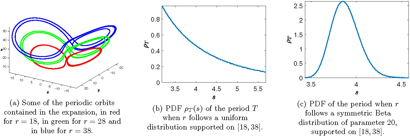
Figure 1: We illustrate here some of the information that can be recovered from the Fourier\(\times\)PC expansion of the random periodic orbit. The computations where done for \(\zeta=10\), \(\beta=8/3\), \(K=80\), \(N=10\) and \(r\) a random variable taking values in the interval \([18,38]\).

Other random invariant sets such as random local stable/unstable manifolds (R2), or random connecting orbits, can be approximated using PCE in a similar fashion, and we refer to [3] for the details.

2.2. Rigorous Validation

One important issue that was ignored in the previous subsection is the one of the accuracy/reliability of the obtained approximation. This is especially relevant because, even for deterministic ODEs and PDEs, simply proving the existence of global solutions like periodic or connecting orbit is often very challenging, at least outside of perturbative/asymptotic parameter regimes, hence guaranteed a posteriori error estimates are typically also lacking.

However, it turns out one can remedy both problems at once, thanks to an a posteriori validation procedure which provides both the existence of a periodic orbit (or of the other types of invariant sets previously mentioned), and an explicit error bound controlling the distance between this solution proven to exist and the approximation computed using a truncated PCE like (2.2).

Starting from the proof of the Feigenbaum conjecture [10], this type of computer-assisted constructive existence results has become more and more common for deterministic problems, in particular in combination with numerical approximations using truncated Fourier series and Chebyshev series [1, 4, 11]. These techniques are based on a kind of Newton-Kantorovich theorem, whose assumptions are checked with a combination of pen-and-paper and numerical computations, the latter being done with interval arithmetic [14, 15] to ensure that even rounding errors are controlled (see e.g. [18] for a broader discussion of the whole procedure). These techniques were generalized in [2] to a wider framework which encompasses several PCE corresponding to probability densities with compact support, like Legendre polynomials (uniform distributions), Gegenbauer polynomials (symmetric Beta distributions), and tensor products of those.

As an example application, the approximate random periodic orbits of the Lorenz system discussed in Section 2.1 (see Figure 1) can be validated. For instance, in the case where \(r\) is assumed to be uniformly distributed in \([18,38]\), we proved the existence of a random periodic solution of (1.2), at a distance less than \(1.4\times 10^{-4}\) (in some weighted \(\ell^1\) norm) from the approximate solution. In particular, we now have access to both an approximate expectation of the period of this random periodic orbit based on the PCE: \(\mathbb{E}(T)\approx 3.9286\), and a guaranteed error bound: \(\left\vert \mathbb{E}(T)- 3.9286\right\vert \leq 4\times 10^{-4}\).

3. Bifurcations for Random ODEs

3.1. Polynomial Chaos Expansion & Bifurcation Type

Polynomial chaos expansions (PCEs) cannot only be used for (rigorous) computational arguments for random invariant sets but also to address random dynamics close to bifurcations. PCE offers one possibility to connect the random setup with already existing theory in the purely deterministic setting [9, 17, 20], where it is known that parameter variations can induce qualitative changes in the structure of the flow. The pitchfork bifurcation is one classical example. In its normal form, i.e. in terms of the locally governing dynamics, it reads as

\( x' = qx \pm x^3. \)

(3.1)

There is a smooth transition to the new equilibrium branch for \(-x^3\) (supercritical pitchfork bifurcation) and a critical transition (passing of a tipping point) occurs for \(+x^3\) (subcritical pitchfork bifurcation).

 

(Left) Subcritical pitchfork bifurcation (\(+x^3\) in (3.1)). (Right) Supercritical pitchfork bifurcation (\(-x^3\) in (3.1)). Click on the animations to see the full size videos.

A pitchfork bifurcation can also be found in the Lorenz system (1.2), for which the origin is always an equilibrium. We take \((p_1,p_2)=(\zeta,\beta)\) as random parameters and \(q=r\) as a deterministic parameter. When we vary \(r\), the origin undergoes a pitchfork bifurcation at \(r=0\), whose criticality is crucially affected by the random parameters \(p\). Using a center manifold reduction [9, Section 5.1], we obtain the following normal form for this pitchfork bifurcation, where the sign of the bifurcation normal form coefficient \(X\) encodes the criticality.

\( u' = \frac{p_1}{1+p_1} q u - \underbrace{\frac{p_1}{p_2(1+p_1)}}_{= X}u^3 -\frac{p_1^2}{(1+p_1)^3} q^2 u + \mbox{higher-order terms}. \)

(3.2)

Details of the reduction step can be found in [8]. A crucial observation is that the random parameters are nonlinearly transformed into \(X\). This is rather generic and not limited to the case of a pitchfork bifurcation. For example, the random parameters might also render the first Lyapunov coefficient into a random variable [7]. The latter determines the criticality of a Hopf bifurcation [9, Section 3.5].

We now address how PCE can be used in the study of random bifurcation coefficients (R3) such as \(X\) in (3.2). In this special case, the probability of \(X\) being positive could be derived from the individual probabilities \(p_1 \in (-\infty,-1) \cup (0,\infty)\) and \(p_2>0\). Note however that, for other nonlinear transformations, it might not be enough to compute independently the probability of each part being positive. Our goal is to determine a method to calculate the probability distribution of \(X\), or at least determine the probability to observe a sub- or a supercritical pitchfork bifurcation.

So we need to calculate (or estimate) the probability distribution of a general nonlinear function \(g(p)\) of random parameters \(p\). In [8], we present three different approaches. Here, we will highlight a semi-analytical, sampling-free procedure that is advantageous if one evaluation of \(g\) is very costly.

It is well-known that the probability distribution of the sum of two independent random variables can be calculated as convolution of the individual distributions. Since, we deal with general nonlinear functions, it would be nice to have an analogous representation for their product. This can be achieved by using the Mellin transform, an integral transform over the positive half-line, defined as a function of the complex variable \(s\in \mathbb{C}\) (cf. [16, p. 96]):

\( \mathcal{M}\left(F(y)\right)(s) = \int_{0}^{\infty} y^{s-1}F(y) dy \)

(3.3)

for a single- and real-valued function \(F\) that is defined almost everywhere for \(y\geq 0\). An inverse Mellin transform can also be defined but an explicit inversion is not always possible. However, there is a useful probabilistic interpretation of the Mellin transform as the \((s-1)\)-th moment, \(s\in \mathbb{N}\), of a random variable, i.e.

\( \mathcal{M}\left(\rho_\xi(x)\right)(s) = \mathbb{E}\left[\xi^{s-1}\right] =: \mathcal{M}(\xi)(s), \)

(3.4)

where \(\xi\) is an almost surely (a.s.) positive random variable on a given probability space with corresponding probability density \(\rho_\xi\). An extension of the Mellin transform to random variables also attaining negative values is described in [5]. The Mellin transform has many useful properties, e.g., for positive independent random variables \(\xi_1,\dots,\xi_n\) we have

\( \mathcal{M}(\prod_{i=1}^{n}\xi_i)(s) = \prod_{i=1}^{n}\mathcal{M}(\xi_i)(s). \)

(3.5)

The Mellin transform of the inverse \(\eta = \frac{1}{\xi}\) of the positive random variable \(\xi\) is

\( \mathcal{M}(\eta)(s) =\mathcal{M}(\xi)(-s+2). \)

(3.6)

For some standard distributions the Mellin transform has a simple explicit form, e.g., for \(\xi_U\sim\mathcal{U}(0,1)\) we have

\( \mathcal{M}\left(\xi_U\right)(s) = \frac{1}{s}, \quad \mbox{for} \ \mbox{Re}(s)>0. \)

(3.7)

but in many other cases, no analytical formula exists. The idea is to decompose the bifurcation coefficient into formula-based part and a remainder. Then, PCE comes into play. We expand the remainder in a PCE and calculate the Mellin transform of the PCE. We combine again both parts and have moments of the bifurcation coefficient available in closed form without sampling. To derive a PDF of the bifurcation coefficient, we use the method of moments (see e.g. [6]). We apply the method to a Gaussian mixture model [13], where its PDF is decomposed into weighted Gaussian component densities. This gives us a lot of flexibility since for example also multi-modal distributions can be captured. We illustrate our semi-analytical approach via the Lorenz system (3.2). We calculate the Mellin transform of \(X\) by applying property (3.5) to obtain

\( \mathcal{M}(X)(s) = \mathcal{M}\left(\frac{{p_1}}{{p_2}(1+{p_1})}\right)(s) = \underbrace{\mathcal{M}\left(\frac{1}{{p_2}}\right)(s)}_{\mbox{analytically tractable}} \cdot \underbrace{\mathcal{M}\left(\frac{{p_1}}{1+{p_1}}\right)(s)}_{\mbox{no analytical expression}}. \)

Assume the uncertain input \(p_1\) follows a generalized Beta distribution supported on \([-0.5,0.5]\) with parameters \((2,5)\), i.e. \(p_1\sim\mbox{Beta}_{-0.5}^{0.5}(2,5)\), and \(p_2\) is Gamma distributed with shape \(8\) and rate \(1\), i.e. \(p_2\sim\Gamma(8,1)\). For the analytical part, via (3.6), we immediately obtain

\( \mathcal{M}\left(\frac{1}{p_2}\right)(s) = \mathcal{M}\left(p_2\right)(-s+2) = \frac{\Gamma(8-s+1)}{\Gamma(8)}. \)

(3.8)

For the remainder, we expand \(g(p_1)=\frac{p_1}{1+p_1}\) into a PCE as done in (2.1). We prefer to work with a uniform stochastic germ \(\xi := \tilde{U} \sim \mathcal{U}(0,1)\) instead of \(p_1\) itself since the Mellin transform of \(\tilde{U}\) has the simple form (3.7). The corresponding orthogonal basis are shifted Legendre polynomials \(\left(\tilde{\phi}_n\right)_{n\geq 0}\), i.e. \(\tilde{\phi}_n(x) = \phi_n(2x-1)\), where \(\left(\phi_n\right)_{n\geq 0}\) are the classical Legendre polynomials. We move to the monomial basis with transformed deterministic coefficients \(\left(c_n\right)_{n\in \mathbb{N}}\) and obtain

\( g(p_i) \approx \sum_{n=0}^{N} g_n\tilde{\phi}_n(\xi) = \sum_{n=0}^{N} c_n \xi^n, \)

(3.9)

The Mellin transform of the reformulated PCE (3.9) for \(s\in \mathbb{N}\) finally reads as

\( \mathcal{M}\left(\sum_{n=0}^{N} c_n \xi^n\right)(s) = \sum_{i=0}^{N\cdot(s-1)} \hat{c}_i(s) \cdot \mathcal{M}(\xi)(i+1), \)

(3.10)

where \(\hat{c}_i(s)\) denote the cumulated coefficients for the powers of \(\xi\). They result from a repeated use of the binomial formula. For the details, we refer to [8].

By putting (3.8) and (3.10) together, we obtain the approximation of the Mellin transform of \(X\) as

\( \mathcal{M}\left(X\right)(s) \approx \frac{\Gamma(8-s+1)}{\Gamma(8)}\cdot \sum_{i=0}^{N\cdot(s-1)} \frac{\hat{c}_i(s)}{i+1}. \)

(3.11)

This is appealing since we now have approximated moments of \(X\) available in the closed form (3.11). By now fitting a Gaussian mixture model via the method of moments (five moments used, truncation \(N=2\)), we obtain the results depicted in Figure 2 (taken from [8, Figure 3]). We obtain that the probability to observe a subcritical pitchfork bifurcation amounts to \(0.9049\) being very close to the standard Monte Carlo estimate of \(0.8903\).

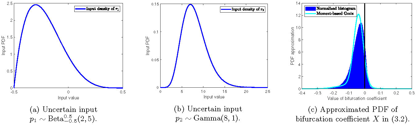
Figure 2: (a): PDF of the input parameter \(p_1\); (b) PDF of the input parameter \(p_2\); (c) Well-designed combination of PCE with Mellin transform gives approximation of moments of \(X\) in (3.11); PDF of Gaussian mixture (Gmix) model (turquoise line) is obtained via a method of moments; good agreement of the PDF with the normalized histogram over \(M=10^6\) samples of \(X\).

3.2. Random Bifurcation Diagrams

Beyond single bifurcation points, an even more ambitious goal would be to study entire random bifurcation diagrams. Another prototypical bifurcation is the fold bifurcation with normal form \(x' = q - x^2\). Here, the transition is always critical, i.e. a fold bifurcation point is a tipping point. In [12], we addressed the visualization of random bifurcation diagrams (R4) resulting from the influence of a random parameter \(p\) in the normal form. We illustrated our analysis via a box model of the Atlantic Meridional Overturning Circulation with an uncertain parameter for the ratio of diffusive to advective timescale. By using a Bayesian inversion approach based on synthetic salinity difference data, we achieved a substantial narrowing of the nature and location of the bifurcation points with respect to the nondimensional freshwater flux. The visualization tools provided therein contribute to a better interpretation of probabilistic tipping behavior; see Figure 3.

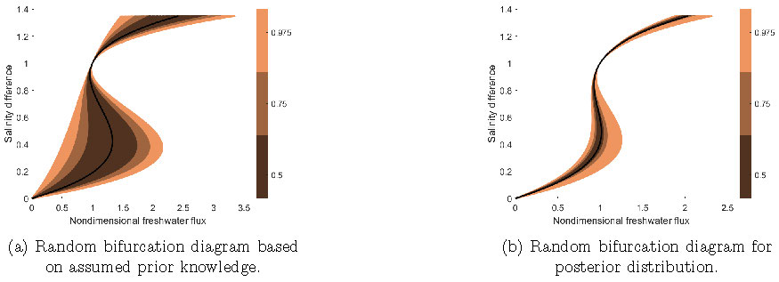
Figure 3: Random bifurcation diagrams for box model of the Atlantic Meridional Overturning Circulation according to prior and posterior parameter distribution from Bayesian inference on synthetic data. We obtain a substantial narrowing of the nature and location of the bifurcation points. Figures adapted from [12] and for further details, also see [12].

4. Summary and Outlook

We have seen that carrying over standard tools from deterministic nonlinear dynamics to RODEs/RPDEs is not always straightforward. Random input parameters turn all objects (R0)-(R4) into random ones. We have presented tools to extract probabilistic nonlinear dynamics information for systems with random parameters, e.g., for computing invariant sets, bifurcation coefficients, or bifurcation diagrams. Yet, there are still many open theoretical problems, e.g., we are actively working on computing coarse-grained observables for random dynamical objects. Thinking about real-world applications, the space of random input parameters RODE/RPDE is likely to be high-dimensional. To tame the complexity, dimension reduction is necessary making the system more accessible for a (semi-)analytical treatment, which is another avenue currently pursued in dynamical systems methods for RODEs.

For the presentation "Uncertainty Quantification of Bifurcations for RODEs" by Kerstin Lux on 27.05.2021 at the SIAM DS Conference, see https://www.youtube.com/watch?v=cbeYtHl5zIM.

References

[1]   G. Arioli and H. Koch, Computer-assisted methods for the study of stationary solutions in dissipative systems, applied to the Kuramoto-Sivashinski equation, Arch. Ration. Mech. Anal., 197 (2010), pp. 1033-1051.

[2]   M. Breden, A posteriori validation of generalized polynomial chaos expansions, arXiv preprint arXiv:2203.02404, 2022.

[3]   M. Breden and C. Kuehn, Computing invariant sets of random differential equations using polynomial chaos, SIAM Journal on Applied Dynamical Systems, 19 (2020), pp. 577-618.

[4]   S. Day, J.-P. Lessard, and K. Mischaikow, Validated continuation for equilibria of PDEs, SIAM J. Numer. Anal., 45 (2007), pp. 1398-1424.

[5]   B. Epstein, Some Applications of the Mellin Transform in Statistics, The Annals of Mathematical Statistics}, 19 (1948), pp. 370-379, https://doi.org/10.1214/aoms/1177730201.

[6]   L. P. Hansen, Generalized Method of Moments Estimation, Palgrave Macmillan UK, London, 2008, pp. 1-10.

[7]   C. Kuehn, Uncertainty transformation via Hopf bifurcation in fast-slow systems, Proc. R. Soc. A, 473 (2017), p. 20160346.

[8]   C. Kuehn and K. Lux, Uncertainty quantification of bifurcations in random ordinary differential equations, SIAM Journal on Applied Dynamical Systems, 20 (2021), pp. 2295-2334.

[9]   Y. A. Kuznetsov, Elements of Applied Bifurcation Theory, vol. 112 of Applied Mathematical Sciences, Springer-Verlag, New York, third ed., 2004, https://doi.org/10.1007/978-1-4757-3978-7.

[10]   O. E. Lanford III, A computer-assisted proof of the Feigenbaum conjectures, Bulletin of the American Mathematical Society, 6 (1982), pp. 427-434.

[11]   J.-P. Lessard and C. Reinhardt, Rigorous numerics for nonlinear differential equations using Chebyshev series, SIAM J. Numer. Anal., 52 (2014), pp. 1-22.

[12]   K. Lux, P. Ashwin, R. Wood, and C. Kuehn, Assessing the impact of parametric uncertainty on tipping points of the atlantic meridional overturning circulation, Environmental Research Letters, 17 (2022), p. 075002, https://doi.org/10.1088/1748-9326/ac7602.

[13]   G. McLachlan and D. Peel, Finite mixture models, Wiley Series in Probability and Statistics: Applied Probability and Statistics, Wiley-Interscience, New York, 2000, https://doi.org/10.1002/0471721182.

[14]   R. E. Moore, Interval analysis, vol. 4, Prentice-Hall Englewood Cliffs, 1966.

[15]   S. M. Rump, Verification methods: Rigorous results using floating-point arithmetic, Acta Numer, 19 (2010), pp. 287-449.

[16]   M. D. Springer, The Algebra of Random Variables, Wiley Series in Probability and Mathematical Statistics, John Wiley & Sons, New York-Chichester-Brisbane, 1979.

[17]   S. H. Strogatz, Nonlinear Dynamics and Chaos, With Applications to Physics, Biology, Chemistry, and Engineering, Westview Press, Boulder, CO, second ed., 2015.

[18]   J. B. van den Berg and J.-P. Lessard, Rigorous numerics in dynamics, Notices Amer. Math. Soc., 62 (2015).

[19]   N. Wiener, The homogeneous chaos, American Journal of Mathematics, 60 (1938), pp. 897-936.

[20]   S. Wiggins, Introduction to Applied Nonlinear Dynamical Systems and Chaos, vol. 2 of Texts in Applied Mathematics, Springer-Verlag, New York, second ed., 2003.

[21]   D. Xiu and G. E. Karniadakis, The Wiener-Askey polynomial chaos for stochastic differential equations, SIAM journal on scientific computing, 24 (2002), pp. 619-644.