Joseph Teran, Scientific Computing for Visual Effects.
1 Introduction
Nowadays, PhD graduates in scientific computing are needed in an exciting new field: movie special effects. Studios like Walt Disney Animation, Industrial Lights and Magic and Pixar increasingly require expertise in the numerical approximation of partial differential equations (PDEs). Specifically, PDEs that describe the dynamics of materials encountered in the scenes of the movie. This includes the mundane like water, dirt, sand, mud, air, even clothing, hair and skin. It also includes the sensational, e.g., fire, explosions, rapid failure etc. Realistic dynamic movement of these types of materials is essential for creating compelling and captivating virtual scenes. These dynamics can be described with PDEs arising from the continuum mechanics form of classical physics, e.g., the Navier-Stokes equations for incompressible fluid dynamics. However, since the equations are highly nonlinear, we cannot solve them exactly, but we can approximate them very accurately using applied mathematics and scientific computing. While approximating a PDE numerically is very computationally expensive and requires an expert user, it is often the only way to get satisfactory behavior at the level of quality demanded by today's motion pictures.
Modern Hollywood blockbusters rely on more and more computer generated (CG) scenery. This is used to composite with live action for movies like Star Wars and the Avengers. For fully animated features like those produced by Walt Disney Animation and Pixar, the entire movie is CG. Computer graphics researchers are traditionally concerned with synthesizing photography of these CG assets to create the frames in the movie and the state-of-the-art has progressed very rapidly. It is often difficult to tell the difference between a real photograph and a rendered scene. This static visual fidelity raises the bar for the realism of the physical dynamics of the materials in the scenes. For example, if a rendered still frame of CG water looks like a photograph, the animated water must move like real water. If it does not, the water appears unnatural and draws the viewer's attention since it looks like water but moves in a manner we do not expect. Everyday common materials are the hardest to get right in terms of dynamics. We have a lot of familiarity with them so it is easier to tell if something is not right. More sensational effects like a building crumbling or an explosion are easier because we are not as familiar with them; more simplifications to the physics and discretization algorithms can be made.
With each passing year and movie, the studios adopt more and more simulation as the demand for realism increases. I will discuss a number of materials that are typically simulated, as well as the PDEs describing their behavior and the numerical methods popularly used to approximate their solution in the effects industry.

Figure 1: Snow business. In Disney's Frozen, snow is simulated as an elastopolastic granular material using the Material Point Method (MPM) [15]. This method naturally reproduces snow cohesion and failure in response to character interaction.

Figure 2: Character animation. The leftmost image shows the underlying skeleton used for animation. The rightmost image shows the polyhedral skin mesh displaced from the animated skeleton. The center image shows the FEM hexahedral mesh used for simulating quasi-static equilibrium.
2 Character animation and clothing
In a fully animated feature like Disney's Frozen or Tangled, each character in the movie is represented geometrically as a polyhedral mesh (see Figure 2). Their hair and clothing are also represented in this way. Animating the characters is done by specifying the trajectory of each one of the vertices in the mesh over time. This task can be very expensive since a mesh will consist of hundreds of thousands to millions of vertices. To expedite the process, artists often control a simplified underlying skeleton with fewer degrees of freedom than the surface mesh (see Figure 2, left). The skin vertex positions must then be extrapolated from the configuration of the underlying skeleton. Physically, the elastic properties of soft tissues like muscle, tendon, ligament and fat determine this extrapolation. This can be described mathematically by a PDE that expresses elastic equilibrium
\begin{equation} \nabla \cdot \bf{P} + \rho \rm{g} = \bf{0} \quad (1) \end{equation}
\begin{equation} \bf{P} = \frac{\partial \psi}{\partial \bf{F}} \quad (2) \end{equation}
\begin{equation} \bf{F}= \frac{\partial \phi}{\partial \bf{X}} \quad (3) \end{equation}
with Dirichlet boundary conditions \( \phi({\bf{X}},t) = \phi_b({\bf{X}},t) \) for \( {\bf{X}} \in \partial\Omega_b^0\) and free surface boundary conditions \( \bf{P}(\bf{X},t)\bf{N}(\bf{x})=\bf{0}\) for \( {\bf{X}} \in \partial\Omega^0\) . Here, \(\phi:\Omega^0\to\Omega^t\) is the flow map of the material that describes where a particle \({\bf{X}} \in \Omega^0\) in the original configuration of the body \(\Omega^0\) is at time \(t\). \(\partial \Omega_b^0\) is the portion of the boundary of the soft tissues in contact with the bones in the skeleton and \(\partial \Omega_s^0\) is the surface of the skin. \( {\bf{F}} = \frac{\partial\phi}{\partial {\bf{X}}}\) is the flow map Jacobian (or deformation gradient), \({\bf{P}} = \frac{\partial \psi}{\partial {\bf{F}}} \) is the first Piola Kirchhoff stress and \(\psi\) is the elastic potential energy density. The elastic potential energy density \(\phi({\bf{F}}) \) penalizes non-rigid motions (or non-orthogonal \({\bf{F}}\)), e.g., \( \psi({\bf{F}}) = \mu |{\bf{F-R(F)}}|_F^2 + \frac{\lambda}{2}({\rm{det}}({\bf{F}})-1)^2 \) is often used, where \({\bf{F=R(F)S(F)}}\) is the polar decomposition of the deformation gradient. The problem is equivalent to minimizing the total elastic potential energy \( e=\int_{\Omega^0}\phi({\bf{F}}({\bf{X}},t))d{\bf{X}} \) subject to the Dirichlet boundary conditions. In a recent paper [14], we showed that these problems can be approximated using the finite difference discretization over a structured hexahedral lattice (see Figure 2, middle).
The finite element method (FEM) could also naturally be used, but our discretization was designed to have a linearization that is more sparse to optimize numerical linear algebra. The discrete system of equations that we derive is nonlinear as a consequence of nonlinearity in the energy density \(\psi\) and we use Netwon's method with multigrid to solve the linearized systems. The method was designed to scale efficiently with many-core parallel implementation and runs nearly in real-time for hexahedral lattices with hundreds of thousands of vertices. Speed of computation is very important and must be nearly real-time in production. Artists typically need many iterations to perfect a character animation for a given scene and these techniques would not be practical with computation that is not nearly real-time.
Once the motion of the character has been animated, its clothing must also be simulated in a post-process (see Figures 3 and 4). Each layer of clothing, e.g., shirt, pants, jacket, socks etc is represented as a polyhedral mesh. Their dynamics must be simulated where the trajectory of the character and its skin are used as hard constraints. Each layer of clothing is simulated as an elastic membrane whose constitutive behavior is similar to that of skin and soft tissue. However, there is also a challenging contact problem between the layers of clothing that must be solved. This is often expressed as a non-penetration constraint for each pair of simple mesh facets like edge/edge and point/triangle. The most common means of satisfying these constraints are with impulsive changes in momentum that happen upon mesh facet collisions as in Bridson et al [5] or via dynamically defined, spring-like potentials that resist penetration as in Baraff and Witkin [1].
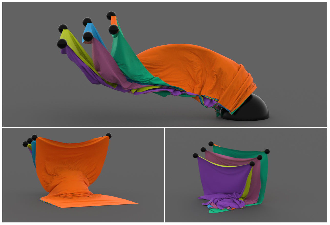
Figure 3: Cloth collisions. The dynamics of each garment that CG characters wear must be simulated to achieve sufficient realism. Physically they are modeled as elastic surfaces, but self and external collisions must also be resolved. Here it is done using MPM and elastoplasticity [9].

Figure 4: Knit fabrics. Recently Jiang et al [9] showed that cloth and knit collisions can be resolved with MPM and elastoplasticity. Here each yarn strand in a knit sweater is simulated and self and external contacts are naturally and efficiently resolved.
3 Water
Water (and more generally incompressible fluid) is one of the most commonly simulated materials in visual effects. The incompressible Euler equations (rather than Navier Stokes) are often used since numerical viscosity is typically comparable to real life. These equations are used to produce effects such as water pouring into a glass, rushing waterfalls and streams, characters splashing and swimming in a pool or ocean, etc. (see Figure 5). As with the PDE for character animation (Equations (1)-(3)), a mix of free surface and Dirichlet boundary conditions is most commonly used:
\begin{equation} \rho ( \frac{\partial {\bf{v}}}{\partial t} + \frac{\partial {\bf{v}}}{\partial x} {\bf{v}} ) = - \nabla p + \rho \rm{g} \quad (4) \end{equation}
\begin{equation} \nabla \cdot {\bf{v}} = 0 \quad (5)\end{equation}
with \(p=0\) at the free surface and \({\bf{v}} = {\bf{v}}_{\partial \Omega_D}\) in the Dirichlet portion of the boundary (where \( {\bf{v}}_{\partial \Omega_D} \)is the velocity of an interacting character and/or external domain). The computational domain \(\Omega\) is typically geometrically complex since it is a part of the world in the movies (e.g., the complement of a wine glass or a river bed in Figure 5). There are many methods in the scientific computing literature that handle these equations in complex geometries, but particle-based approaches have proven to be the most popular in the effects industry. Artists generally appreciate the intuitive and familiar nature of Lagrangian particles and methods that use them are very popular. Particle representations are simple to incorporate into other aspects of the production pipeline and there are many existing tools that can be used to artistically direct and manipulate them. Bridson and colleagues [17, 4, 2, 6] demonstrated the efficacy of the hybrid Lagrangian/Eulerian Particle-In-Cell (PIC) method of Harlow [7] for graphics applications. These have become the industry standard. Specifically, the Fluid-Implicit-Particle (FLIP) improvement to PIC developed by Brackbill is the key to its adoption since it removes otherwise excessive dissipation [3].
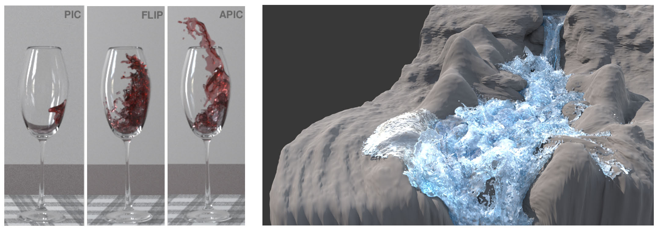
Figure 5: Incompressible flow. Incompressible flow is widely used to model fluids like water, wine, etc. The nature of the workflow in movie production places rather unique demands on algorithms including geometric flexibility, computational efficiency and natural artistic controllability.
Most techniques used in effects are based on equation splitting as in, e.g., Harlow and Welch [8]:
\begin{equation} \frac{{\bf{v}}^*-{\bf{v}}^n}{\Delta t} + \frac{\partial {\bf{v}}^n} {\partial {\bf{x}}} {\bf{v}}^n = {\bf{g}} \quad (6) \end{equation}
\begin{equation} \frac{{\bf{v}}^{n+1}-{\bf{v}}^*}{\Delta t} + \nabla p^{n+1} = 0 \quad (7) \end{equation}
\begin{equation} \nabla \cdot {\bf{v}}^{n+1} = 0 . \quad (8) \end{equation}
In this case the pressure can be decoupled from the velocity using the intermediate velocity \({\bf{v}}^*\). The intermediate velocity is determined from advection and gravity alone. The pressure is then isolated as a Lagrange multiplier that enforces incompressibility of the final velocity \({\bf{v}}^{n+1}\):
\begin{equation} {\bf{v}}^* = {\bf{v}}^n - \Delta t \frac{\partial {\bf{v}}^n}{\partial {\bf{x}}} v^n + \Delta t {\bf{g}} \quad (9) \end{equation}
\begin{equation} \nabla \cdot {\bf{v}}^* = \Delta t \Delta p^{n+1} \quad (10) \end{equation}
\begin{equation} {\bf{v}}^{n+1} = {\bf{v}}^* - \Delta t \nabla p^{n+1}. \quad (11) \end{equation}
As in Harlow and Welch [8], a staggered marker and cell (MAC) grid is typically used to prevent pressure checker-boarding with centered stencils. A MAC grid stores velocities at faces of a regular Cartesian lattice (see Figure 6, left). Pressures are stored at cell centers. The solution of the Poisson problem in Equation (10) in the irregular domain of the fluid is typically the bottleneck in this process and much work has been done to develop efficient solvers and preconditioners [13].
The PIC/FLIP approach is primarily a means of solving the advection in Equation (9). The primary state is Lagrangian and the fluid is represented by marker particles with positions \({\bf{x}}_p^n\) and velocities \({\bf{v}}_p^n\) . Mass and mass density are typically not used since \(\rho = 1\) holds for all time when it holds initially and there is satisfaction of the incompressibility constraint. With this view, the advection step in the split Equations (9) is approximated with simple Lagrangian particle motion and transfers back and forth between particles and grid:
\begin{equation} w_{i_\alpha}^n = N({\bf{x}}_p^n - {\bf{x}}_{{\bf{i}}_\alpha}) \quad (12) \end{equation}
\begin{equation} v_{\alpha {\bf{i}}_\alpha}^* = \frac{1}{\sum_q w_{{\bf{i}}_\alpha q}^n} \sum_p v_{\alpha p}^n w_{\bf{i}\alpha P}^n \quad (13) \end{equation}
\begin{equation} \nabla^{\Delta x} \cdot {\bf{v}}^* = \Delta t \Delta^{\Delta x}p^{n+1} \quad (14) \end{equation}
\begin{equation} {\bf{v}}^{n+1} = {\bf{v}}^* - \Delta t \nabla^{\Delta x}p^{n+1} \quad (15) \end{equation}
\begin{equation} v_{\alpha p}^{n+1} = v_{\alpha p}^n + \sum_{{\bf{i}}_\alpha} \big(v_{\alpha {\bf{i}}_\alpha}^{n+1} - v_{\alpha {\bf{i}}_\alpha}^* \big) w_{ {\bf{i}}_\alpha p}^n \quad (16) \end{equation}
\begin{equation} x_{\alpha p}^{n+1} = x_{\alpha p}^n + \Delta t \sum_{{\bf{i}}_\alpha} v_{\alpha {\bf{i}}_\alpha}^{n+1} w_{{\bf{i}}_\alpha p}^n. \quad (17) \end{equation}
Here the weights \(w_{{\bf{i}}_\alpha} = \sum_P N(x_p^n-x_{{\bf{i}}_\alpha}) \) are defined from B-spline interpolating functions over a Cartesian grid. The \( x_{{\bf{i}}_\alpha}\) are the nodes of the staggered velocity grid associated with velocity component \(\alpha\) (see Figures 6 and 7) where \({\bf{i}}_\alpha \) is the index in the grid of the node. \( v_{\alpha i_\alpha}^* \) is the \(\alpha \) component of the grid velocity before projection. \( v_{\alpha p}^n \) is the \( \alpha \) component of \( {\bf{v}}_p^n \) with similar conventions for \( v_{\alpha i_\alpha}^{n+1} \), \( v_{\alpha p}^{n+1} \), \( x_{\alpha p}^{n+1} \), etc. Steps (12)-(13) transfer (extrapolate) Lagrangian particle velocities \( {\bf{v}}_p^n \) to the grid velocities \( {\bf{v}}^* \), steps (14)-(15) project (via solution of Poisson) grid velocity \( v^* \) to its nearest divergence free counterpart \( {\bf{v}}^{n+1} \), and steps (16)-(26) update (interpolate) the particle positions and velocities from the grid.
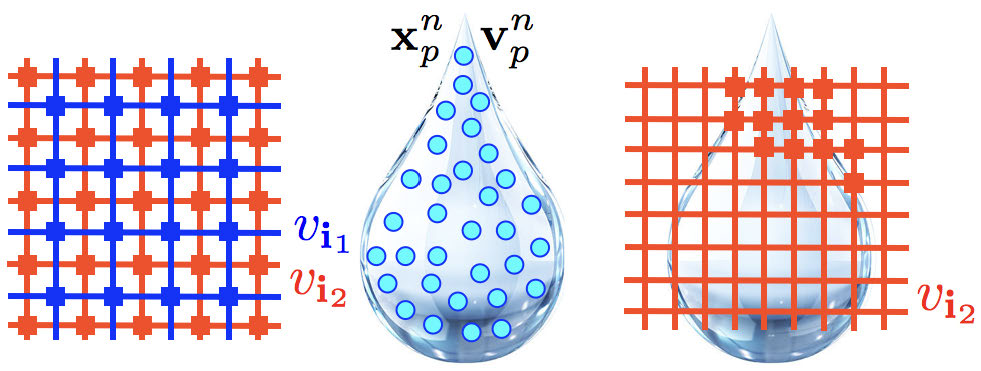
Figure 6: PIC/FLIP and MAC grids. PIC techniques are hybrid Lagrangian/Eulerian and require transferring back and forth between particle and grid representations. For incompressible flow, it is useful to stagger the different components of the grid velocities on different grids.
While Poisson-based pressure projection in Equations (14)-(15) is typically the bottleneck, care must be taken to implement the transfers in Equations (12)-(13) and (16)-(26) efficiently with many-core level parallelism. Practical use of this method for effects production requires simulation with tens to hundreds of millions of particles. We have recently done research developing new versions of these transfers in [10, 11].
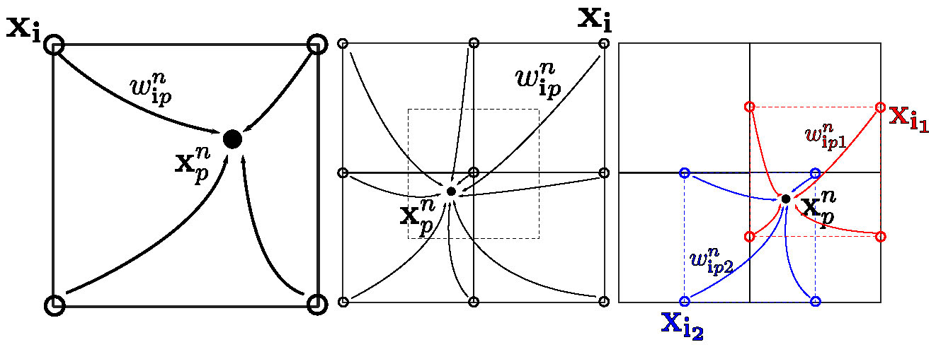
Figure 7: PIC particle/grid transfers. PIC techniques require transferring back and forth between particle and grid representations. Simple interpolating functions defined over structured grids provide the mechanism for doing this.
Material Point Methods
The production and practical art direction requirements of the snow simulation algorithm needed for Disney's Frozen were similar to those for water and incompressible fluids. Given the popularity of PIC for incompressible fluids in the effects industry, Stomakhin et al [15] investigated the use of a PIC technique for snow simulation in Frozen (see Figures 1 and 8). The Material Point Method (MPM) is a generalization of the PIC ideas for history-dependent materials. It was developed by Sulsky et al [16]. Snow constitutive behavior varies with environmental factors, but for characters walking through dry to wet snow, it can accurately be described as an elastoplastic granular material.
Elastoplastic material behavior in the presence of large deformation is characterized by a multiplicative decomposition of the deformation gradient \( {\bf{F}}=\frac{\partial \phi}{\partial {\bf{X}}}\) (recall that \(\phi\) is the flow map of the material):
\begin{equation} {\bf{F}} = {\bf{F}}^E {\bf{F}}^P. \quad (18) \end{equation}
With this convention, the local elastic rest state varies with time and its Jacobian is characterized by the \({\bf{F}}^E\) term. The \({\bf{F}}^P\) term is the Jacobian of the mapping from the initial rest state to the plastically modified rest state. E.g., for perfectly elastic materials like the skin in Equations (1)-(3), \({\bf{F}}^P={\bf{I}}\) . For plastic materials, the deformation in \({\bf{F}}^P\) is permanent and is forgotten elastically. E.g., consider a snow-covered ground after a snowfall. It behaves elastically and retains its shape; however, as someone walks through it, the impact of their feet causes deformation beyond the elastic limit and their footprints are tracked in \({\bf{F}}^P\). The PDEs that express this material behavior are
\begin{equation} \rho \frac{\partial^2 \phi}{\partial t^2} = \nabla \cdot {\bf{P}} + \rho \rm{g} \quad (19) \end{equation}
\begin{equation} {\bf{P}} = \frac{\partial \phi}{\partial {\bf{F}}^E} ({\bf{F}}^E,{\bf{F}}^P) {\bf{F}}^{P^{-T}} \quad (20) \end{equation}
with boundary conditions analogous to skin and water: \(\phi({\bf{X}}, t)\) = \( \phi_b({\bf{X}},t) \) for \( {\bf{X}} \in \partial \Omega_b^0\) and free surface boundary conditions \({\bf{P}}({\bf{X}}, t) {\bf{N(X)}} = {\bf{0}}\) for \({\bf{X}} \in \partial \Omega_s^0\). As with water, \(\Omega_s^0\) is the free surface of the snow and \(\Omega_b^0\) is the boundary of the computational domain (including where scripted characters are moving). We use the elastic energy density \( \psi({\bf{F}}^E,{\bf{F}}^P) = \mu(J^P) |{\bf{F}}^E-{\bf{R}}({\bf{F}}^E)|_F^2 + \frac{\lambda(J^P)}{2}({\rm{det}}({\bf{F}}^E)-1)^2) \), where \(J^P={\rm{det}}({\bf{F}}^P)\), \( \mu(J^P) = \mu^0\epsilon^{-\xi(J^P-1)}\), and \(\lambda(J^P) = \lambda^0e^{-\xi (J^P-1)}\). This is very similar to the elastic energy density used for skin, but where only deformation in the elastic part \({\bf{F}}^E\) is penalized. However, the material gets stiffer or weaker (increasingly with \(\xi\)) as the plastic deformation loses or gains volume respectively. This allows for the stiffening effect of “packing" a snowball, etc.
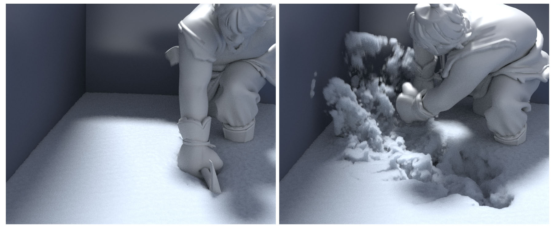
Figure 8: More snow business. Christoph from Disney's Frozen digs in deep snow. The dynamics are simulated with the MPM approach in [15].
The MPM discretization of these equations can be viewed as an updated Lagrangian procedure, where the time \(t_n\) configuration is used as a reference configuration. As with PIC/FLIP and water, the primary state is Lagrangian with particles storing positions \({\bf{x}}_p^n\) and velocities \({\bf{v}}_p^n\). However, unlike water, mass must also be stored per particle \(m_p\), although it does not change with time in accordance with conservation of mass. Additionally, each particle must store the deformation gradient \({\bf{F}}_p^n\) as well as its plastic decomposition \( {\bf{F}}_p^{E,n},{\bf{F}}_p^{P,n} ({\bf{F}}_p^n={\bf{F}}_p^{E,n}{\bf{F}}_p^{P,n}) \). Lastly, each particle must store a volume sample associated with the particle in the initial configuration \(\Delta V_p^0\). With this convention, the state is updated with a loop that is ultimately similar to the original PIC/FLIP for water:
\begin{equation} w_{{\bf{i}}p}^n=N(x_p^n-{\bf{x_i}}) \quad (21) \end{equation}
\begin{equation} m_{\bf{i}}^n=\sum_p m_p w_{{\bf{i}}p}^n \quad (22) \end{equation}
\begin{equation} {\bf{v}}_{\bf{i}}^n=\frac{\sum_p m_p {\bf{v}}_p^n w_{{\bf{i}}p}^n}{m_{\bf{i}}^n} \quad (23) \end{equation}
\begin{equation} {\bf{v_i}}^{n+1}={\bf{v}}_{\bf{i}}^n-\Delta t \frac{1}{m_{\bf{i}}^n} \sum_p {\bf{P}}_p {\bf{F}}_p^n \nabla N ({\bf{x}}_p^n-{\bf{x}}_{\bf{i}}) \Delta V_p^0 + \Delta t {\rm{g}} \quad (24) \end{equation}
\begin{equation} {\bf{v}}_p^{n+1} = {\bf{v}}_p^n + \sum_{\bf{i}} w_{{\bf{i}}p}^n ({\bf{v}}_{\bf{i}}^{n+1} – {\bf{v}}_{\bf{i}}^n) \quad (25) \end{equation}
\begin{equation} {\bf{x}}_p^{n+1} = {\bf{x}}_p^n + \Delta t \sum_i w_{{\bf{i}}p}^n {\bf{v}}_{\bf{i}}^{n+1} \quad (26) \end{equation}
\begin{equation} {\bf{F}}_p^{n+1} = \hat{{\bf{F}}}_p^{n+1} {\bf{F}}_p^n \quad (27) \end{equation}
\begin{equation} [{\bf{F}}_p^{E,n+1},{\bf{F}}_p^{P,n+1}] = {\rm{Clamp}}({\bf{F}}_p^{n+1},{\bf{F}}_p^{P,n}). \quad (28) \end{equation}
Here the grid momentum update in Equation (24) takes the place of the Poisson pressure projection in Equations (14)-(15). The deformation gradient update in Equation (27) is derived from an updated Lagrangian assumption where the deformation \({\bf{F}}_p^{n+1}\) is the product of the deformation from the time \(t^n\) to time \(t^{n+1}\) configuration, \(\hat{{\bf{F}}}_p^{n+1}\) times the deformation at time \(t^n\), \({\bf{F}}_p^n\). Lastly, the plasticity model simply states that the singular values \(\sigma_i^E\) of \({\bf{F}}^E\) must be within a range \(\sigma_i^E \in [1-\theta_c,1+\theta_s]\).
This relatively simple algorithm was used to simulate the interactions of the characters in Frozen with snow in their surroundings (see Figures 1 and 8). Although simplistic, the elastoplasticity model is capable of capturing a wide range of realistic snow behaviors. MPM simulation of more general elastoplastic materials has proven very useful for other applications in the field including sand, mud, dirt (see Figure 9), even knit garments and clothing contact can be modeled as elastoplastic (see Figures 3 and 4).
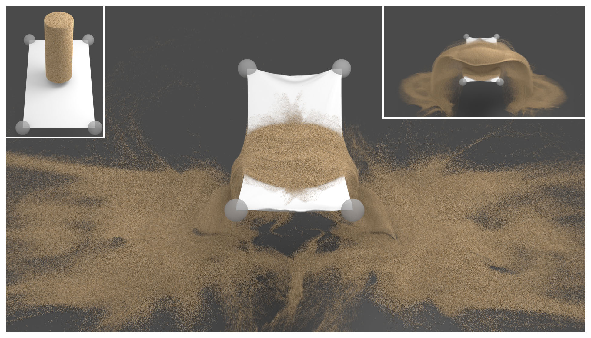
Figure 9: Beyond snow. More general elastoplastic models can be simulated with MPM. Klar et al. [12] investigate the use of the Drucker-Prager yield surface for dry sand.
4 Conclusion
These are just a few of the many PDEs and numerical methods that are used in modern movie special effects. It is truly an exciting and new application area for scientific computing researchers. The demands for realism and efficiency in movie production are always increasing. There is no shortage of algorithmic, mathematical and programming challenges for tomorrow's scientific computing researchers.
References
[1] D. Baraff and A. Witkin. Large steps in cloth simulation. In Proc ACM SIGGRAPH, SIGGRAPH '98, pages 43-54, 1998.
[2] C. Batty, F. Bertails, and R. Bridson. A fast variational framework for accurate solid-fluid coupling. ACM Trans Graph, 26(3), 2007.
[3] J. Brackbill and H. Ruppel. FLIP: A method for adaptively zoned, particle-in-cell calculations of fluid flows in two dimensions. J Comp Phys, 65:314-343, 1986.
[4] R. Bridson. Fluid simulation for computer graphics. Taylor & Francis, 2008.
[5] R. Bridson, R. Fedkiw, and J. Anderson. Robust treatment of collisions, contact and friction for cloth animation. ACM Trans Graph, 21(3):594-603, 2002.
[6] E. Edwards and R. Bridson. A high-order accurate particle-in-cell method. Int J Numer Meth Eng, 90:1073-1088, 2012.
[7] F. Harlow. The particle-in-cell method for numerical solution of problems in fluid dynamics. Meth Comp Phys, 3:319-343, 1964.
[8] F. Harlow and E. Welch. Numerical calculation of time-dependent viscous incompressible flow of fluid with free surface. Phys Fl, 8(12):2182{2189, 1965.
[9] C. Jiang, T. Gast, and J. Teran. Anisotropic elastoplasticity for cloth, knit and hair frictional contact. ACM Trans Graph, 36(4):152:1-152:14, 2017.
[10] C. Jiang, C. Schroeder, A. Selle, J. Teran, and A. Stomakhin. The affine particle-in-cell method. ACM Trans Graph, 34(4):51:1-51:10, 2015.
[11] C. Jiang, C. Schroeder, and J. Teran. An angular momentum conserving affine-particle-in-cell method. J Comp Phys, 338:137-164, 2017.
[12] Gergely Klar, Theodore Gast, Andre Pradhana, Chuyuan Fu, Craig Schroeder, Chenfanfu Jiang, and Joseph Teran. Drucker-Prager elastoplasticity for sand animation. ACM Trans Graph, 35(4), July 2016.
[13] A. McAdams, E. Sifakis, and J. Teran. A parallel multigrid Poisson solver for fluids simulation on large grids. In Proc 2010 ACM SIGGRAPH/Eurograph Symp Comp Anim, pages 65-74. Eurographics Association, 2010.
[14] A. McAdams, Y. Zhu, A. Selle, M. Empey, R. Tamstorf, J. Teran, and E. Sifakis. Efficient elasticity for character skinning with contact and collisions. ACM Trans Graph, 30(4):37:1-37:12, July 2011.
[15] A. Stomakhin, C. Schroeder, L. Chai, J. Teran, and A. Selle. A material point method for snow simulation. ACM Trans Graph, 32(4):102:1-102:10, 2013.
[16] D. Sulsky, Z. Chen, and H. Schreyer. A particle method for history-dependent materials. Comp Meth App Mech Eng, 118(1):179-196, 1994.
[17] Y. Zhu and R. Bridson. Animating sand as a fluid. ACM Trans Graph, 24(3):965-972, 2005.