Bifurcation theory allows the classification of "what typically happens" upon turning one or more "knobs" (or varying parameters) of a dynamical model. For example (under smoothness and nondegeneracy assumptions) a pair of equilibria is generically created upon variation of a parameter in a saddle-node bifurcation when a vector field vanishes at a point where its stability matrix has a zero eigenvalue. If there is a reflection symmetry, then a pitchfork bifurcation can occur, a splitting of two new equilibria away from one. A transcritical bifurcation corresponds to where two equilibria pass through the same point to then re-emerge with exchanged stability. Finally, a Hopf bifurcation creates a limit cycle when a pair of eigenvalues pass through the imaginary axis. These are "local" bifurcations, since everything can be studied in a neighborhood of a special phase space point.

Such basic bifurcations are explained in Steve Strogatz's iconic text "Nonlinear Dynamics and Chaos" [Str15]. However, in Chapter 3, one finds the following problem:

3.4.12 ("Quadfurcation") With tongue in cheek, we pointed out that the pitchfork bifurcation could be called a "trifurcation," since three branches of fixed points appear for \(r >0\). Can you construct an example of a "quadfurcation" ...?

This is a fun problem to assign in class, especially since the answers can be quite varied and not always what (we imagine) the author must have had in mind. Our answer requires the creation of four fixed points from none at a single location in phase space upon variation of one parameter. An answer---for the case of discrete time---is shown in Figure 1(a).

As far as we are aware, the notion of quadfurcation has not occurred otherwise in the dynamical systems literature (however, this term---and the related, if less succinct, "quadrifurcate"---is used in medical literature for a branching of coronary arteries [Hak04]).

One reason might be is that the solution presented in Figure 1(a) requires control of three parameters (the first three derivatives), and that is quite a bit of knob-turning!

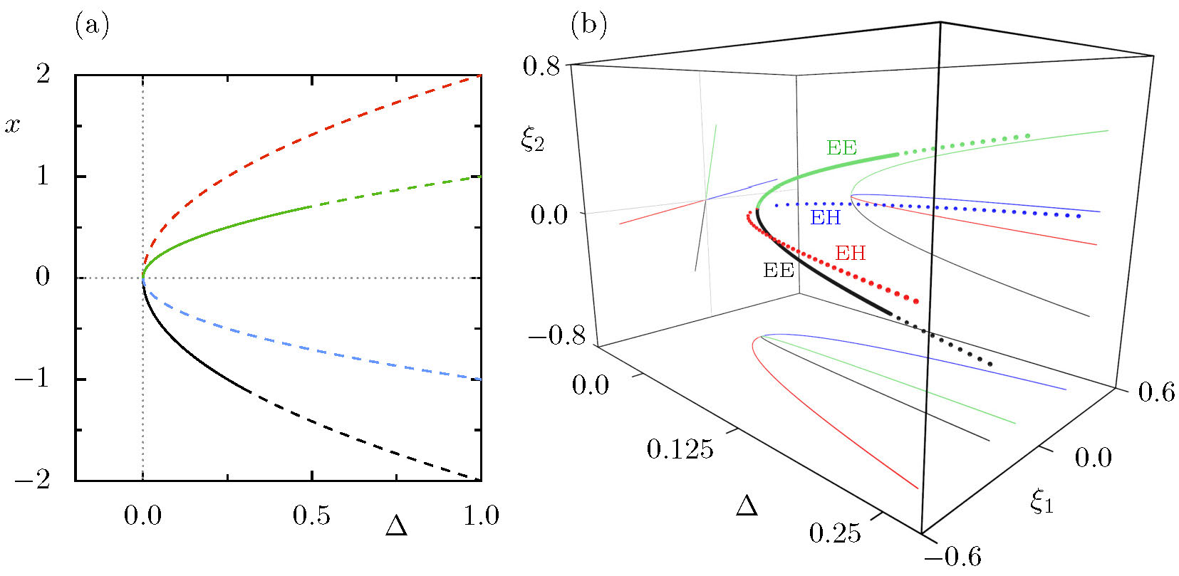
Figure 1. (a) A quadfurcation creates four fixed points of the 1D map \(x' = f(x) = x + (\Delta-x^2)(4\Delta-x^2)\) as \(\Delta\) passes through zero. The two stable fixed points (solid lines) eventually become unstable (dashed lines) by period-doubling. (b) A quadfurcation for Moser's map on the path \((a,b,c) = -\Delta(1.5,0.3,1)\).

Nevertheless, we claim that such a bifurcation is an organizing center for the dynamics of a four-dimensional map [BM18], the quadratic diffeomorphism introduced by Moser in 1994 [Mos94]. Let's begin with the 2D case: Hénon showed in 1976 that the general quadratic diffeomorphism has a normal form with only one quadratic term. This map, with dissipation, has a horseshoe-shaped strange attractor that has become one of the icons of chaos. For the conservative case, Hénon's map can be written in the second difference (or Lagrangian) form,

\((x_{t+1}-x_{t}) - (x_t - x_{t-1}) = a + x_t^2 .\)

(1)

This is an elementary discretization of an oscillator \(\ddot{x} = V'(x)\) with cubically nonlinear potential \(V\). There is only one parameter, \(a\), and the map has a pair of fixed points, born at \(a = 0\), that continue to \(a<0\). This bifurcation creates a saddle---a fixed point with a pair of real eigenvalues---and a center, with a pair of complex eigenvalues on the unit circle. This conservative map, more typically written in canonical variables by defining the momentum \(y_t = x_{t-1}\), is perhaps the simplest representative of a Hamiltonian system that exhibits chaos. Indeed it describes the dynamics near a periodic orbit of a two degree-of-freedom Hamiltonian, using a Poincaré section. Moreover, since any smooth map of the plane can be locally expanded in a power series, (1) gives the local form of the dynamics near a typical fixed point of an area-preserving map.

Moser's generalization of the Henon map has a pair of coordinates \((\xi_1,\xi_2)\in {\mathbb{ R}}^2\) and can be written [BM18] in a similar form

\(C^T (\xi_{t+1}-\xi_t) - C(\xi_t - \xi_{t-1}) = \nabla U(\xi_t) .\)

(2)

Here \(U\) is the potential

\(U = a\xi_1 + b\xi_2 + \tfrac12 c \xi_1^2+ \varepsilon_2 \xi_1^3 + \xi_1 \xi_2^2 ,\)

and \(C\) is a \(2 \times 2\) matrix. This map has two discrete parameters, \(\det(C) = \varepsilon_1 \in \{-1,1\}\), and \(\varepsilon_2 \in \{-1,0,1\}\) and six continuum parameters: the \(a,b,c\) of \(U\) and three elements of \(C\). Of course this second difference equation on \({\mathbb{ R}}^2\) can be rewritten as a map on \({\mathbb{ R}}^4\), and indeed becomes a symplectic map if one defines the momenta \(\eta_{t} = C \xi_{t-1}\). The map is the generic local form for a three degree-of-freedom Hamiltonian flow on a Poincaré section.

Moser's map has, at most, four fixed points (apart from a special case if \(\varepsilon_2 = 0\)). These coalesce at the origin when \(a=b=c=0\): a quadfurcation! The structure depends in detail on the discrete parameters [BM18]; here we suppose that \(\varepsilon_1 = +1\) for simplicity. Consider a path, like \((a,b,c) = -\Delta(1.5,0.3,1)\) that passes through the origin; then when \(\Delta < 0\) there are no fixed points, and when \(\Delta > 0\) there are four, see Figure 1(b). This quadfurcation is an organizing center for the dynamics of Moser's map.

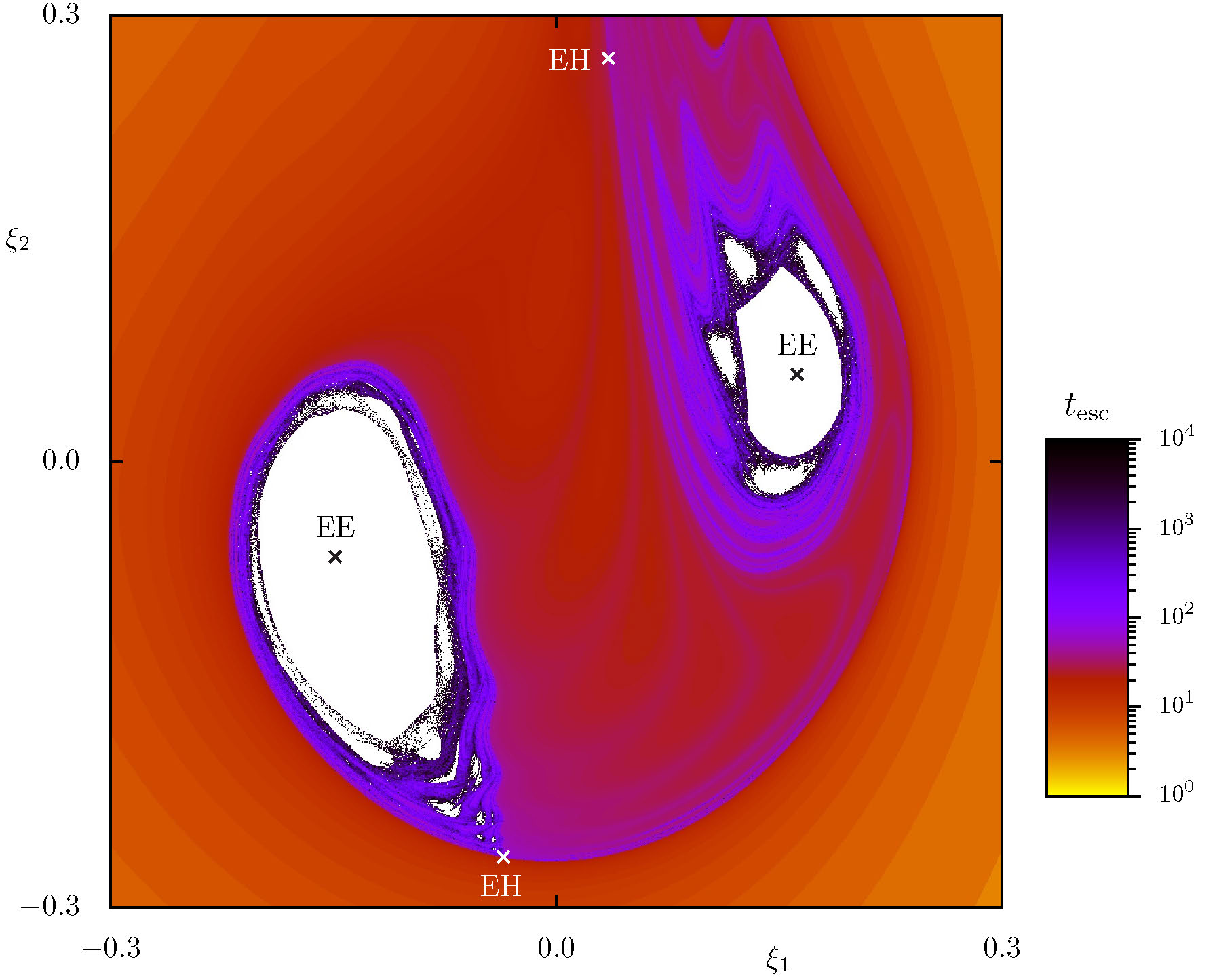
Figure 2. Escape time for orbits of the map (2) for initial conditions in the 2D plane \((\xi,\eta) = (\xi,C\xi)\) that contains all four fixed points. Parameters are \(\varepsilon_1 = \varepsilon_2 = 1\) and \((a,b,c) = (-0.076,-0.019,-0.038)\), with \(C = [1,1.366;-0.366,0.5]\). Orbits are iterated up to \(10^4\) steps, and those that have not yet escaped are colored white.

Just like for the Hénon map, many orbits of Moser's map are unbounded, and families of bounded orbits are associated with stable fixed points. Since (2) is Lagrangian, it cannot have asymptotically stable fixed points; a linearly stable fixed point is doubly elliptic (EE), with four eigenvalues on the unit circle. The local linear dynamics is conjugate to a pair of rotations. When the frequencies are sufficiently irrational, and the nonlinear terms give rise to anharmonicity (i.e., nondegenerate twist), then Kolmogorov-Arnold-Moser (KAM) theory implies there will be many invariant 2D tori in the neighborhood of an EE point. There are two typical scenarios that create EE points for the Moser map. One corresponds to the transition

\(\emptyset \to 2\mbox{ EE} + 2\mbox{ EH},\)

(3)

that creates two doubly elliptic points, and two points (EH) that have one elliptic and one hyperbolic pair (i.e., \(\lambda, \lambda^{-1} \in {\mathbb{ R}}^+\)) of eigenvalues; this is the case shown in Figure 1(b). A second case, which can occur only if \(C\) is symmetric, is the transition

\(\emptyset \to \mbox{ EE} + \mbox{ HH} + 2\mbox{ EH},\)

creating a just one doubly elliptic point and a point (HH) that has two hyperbolic pairs of eigenvalues. This case is perhaps more intuitive; indeed, a four-dimensional map consisting of a pair of uncoupled, 2D maps will have this transition and not the more typical (3).

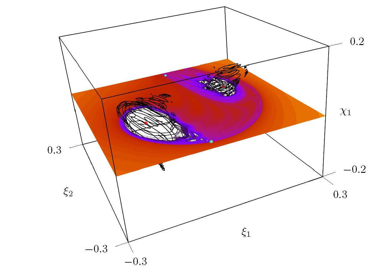
Figure 3. 3D slice of Moser's map with parameters of Figure 2. The small spheres show two EE (red) and two EH (green) fixed points. Also shown are several selected regular tori (black lines) surrounding the EE fixed points, and the escape time plane for \(\chi_1 = 0\) of Figure 2. Each torus is represented by \(10^4\) points in the slice with \(\epsilon=10^{-6}\).

Visualization of dynamics in four dimensions is challenging. One helpful technique is to plot some scalar property of orbits on 2D planes of initial conditions. Common properties include maximal Lyapunov exponents or the "Fast Lyapunov Indicator" (FLI) [LGF16]. Another orbit property is escape time from a region, and when \(\varepsilon_2 \neq 0\), there is a 4D box containing all bounded orbits of (2) [BM18]. Figure 2 shows an example of the structures that occur just after a quadfurcation of type (3). The four fixed points are indicated by \(\times\)'s, and the colors indicate the escape time for initial conditions on a grid of \(3000\times3000\) initial conditions. Near the EE points there are many orbits that appear bounded, but Arnold diffusion should allow trajectories arbitrarily close to the EE fixed points to escape on an exponentially long time scale.

Another visualization technique is the 3D slice [RLBK14]. Consider a 3D hyperplane in the 4D phase space defined by fixing one of the coordinates, e.g., define \(\chi = \eta - C\xi\) and set \(\chi_2 = 0\). The slice is this plane thickened by \(\epsilon\): \[\Gamma = \left\{ (\xi_1, \xi_2, \chi_1, \chi_2)\,|\, |\chi_2| \le \epsilon \right\}.\] Whenever the points of an orbit fall in \(\Gamma\), the remaining coordinates \((\xi_1, \xi_2, \chi_1)\) are displayed in a 3D plot, e.g., Figure 3. When \(\epsilon \ll 1\) one must compute long trajectories in order for some to enter the slice, but the resulting structures appear less fuzzy. A two-torus that intersects the slice will typically appear as two loops. The invariant tori surrounding EE points can be classified by their frequency vectors, and as the frequencies change they undergo various bifurcations creating additional periodic orbits and island structures [RLBK14].

A better understanding of the geometry of these structures will help to analyze Hamiltonian models in such applications as molecular dynamics, long-time storage in particle accelerators, and the trajectories of stars in galaxies.

Funding: JDM was supported in part by NSF grant DMS-1812481 and AB acknowledges support by the Deutsche Forschungsgemeinschaft under grant KE 537/6--1.

References

[BM18]   A. Bäcker and J. D. Meiss, Elliptic bubbles in Moser's 4D quadratic map: The quadfurcation, 2018, https://arxiv.org/abs/1807.06074.

[Hak04]   J. Hakim, Quadfurcation of the left main coronary artery: Double ramus medianus coronary system, Angiology, 55(1), 2004, pp. 109--110, https://doi.org/10.1177/000331970405500118.

[LGF16]   E. Lega, M. Guzzo, and C. Froeschlé, Theory and applications of the Fast Lyapunov indicator (FLI) method, In C. Skokos, G. A. Gottwald, and J. Laskar, editors, Chaos Detection and Predictability, volume 915 of Lecture Notes in Physics, Springer, Heidelberg, 2016, pp. 35--54, https://doi.org/10.1007/978-3-662-48410-4.

[Mos94]   J. K. Moser, On quadratic symplectic mappings, Math. Zeitschrift, 216 (1994), pp. 417--430, https://doi.org/10.1007/BF02572331.

[RLBK14]   M. Richter, S. Lange, A. Bäcker, and R. Ketzmerick, Visualization and comparison of classical structures and quantum states of four-dimensional maps, Phys. Rev. E, 89(2), 2014, p. 022902, https://doi.org/10.1103/PhysRevE.89.022902.

[Str15]   S. H. Strogatz, Nonlinear Dynamics and Chaos: With Applications in Physics, Biology, Chemistry, and Engineering, Studies in Nonlinearity, Westview Press, 2nd edition, 2015.