The peer-reviewed manuscript Swing Shift: a mathematical approach to defensive positioning in baseball was published online in the Journal of Quantitative Analysis in Sports in September 2020 and is scheduled to appear in a future print issue. https://doi.org/10.1515/jqas-2020-0027

This work was also selected for the 2020 MIT Sloan Sports Analytics Conference. http://www.sloansportsconference.com/2020-conference/2020-research-paper-finalists-posters/

Introduction

The sports world and life in general have been turned upside down by the COVID-19 pandemic. With safety precautions in place to protect players, coaches, staff, and fans, sports have gradually been able to return to stadiums, fields, and arenas. In an example of safety precautions entering athletic competition, Major League Baseball player Anthony Rizzo, first baseman for the Chicago Cubs, actually offered a squirt of hand sanitizer to an opposing team’s player who had just reached first base. Fellow first baseman Freddie Freeman of the Atlanta Braves had his own battle with the virus several weeks earlier. These players were notable to us before they were making pandemic-related sports headlines because we used them as test cases in our work exploring a mathematical approach to defensive positioning in baseball.

As baseball fans will tell you, there has been a lot of talk in recent years about a baseball strategy called a shift. A shift refers to the defensive positioning of fielders in non-traditional ways. While a traditional placement involves four infielders and three outfielders, all somewhat evenly spaced, a shift involves overloading one side of the field to account for individual batters’ tendencies. A common use of the shift is to place three infielders all on the right side of the field against left-handed batters since many such batters then to hit to the right.

The aim of this work is to provide possible batter-specific improvements and refinements of shifted positions. We develop an optimization approach that uses integer programming to suggest the placement of seven fielders given a batter’s historic distribution of balls put in play. We only work with seven fielders as opposed to all nine, since the pitcher and the catcher have fixed positions. Not only does our model incentivize coverage of areas with a high density of balls in play for a given batter, but it also penalizes leaving areas of the field open that are likely to result in extra-base hits.

This framework is meant to be a decision-making tool to analytics-minded baseball personnel. The idea is that a user can decide how much they value mitigating the risk of covering extra-base hits versus covering likely areas in which a particular batter is going to put a ball into play. Since the input is at the individual batter level, a coach could run different fielding scenarios for an opponent in an upcoming game to enhance their decision-making ability regarding the best defensive positioning for different game scenarios. The underlying mathematical problem of determining where to place fielders in a baseball field has similarities to facilities location problems in operations research, so this concept can be translated to seemingly unrelated applications through the common mathematical framework.

Mathematical Model

For each point in the baseball field that is beyond a 75-ft radius of home plate, we discretize the field into patches that are approximately 5 ft by 5 ft in size. Each patch has the opportunity to get a player assigned to stand in the patch to start a play, which aligns with the binary decision variable \(x_j\), where

\(x_j=\cases{1, \mbox{if a fielder is assigned to patch } j\cr 0, \mbox{otherwise.}} \)

For the discretization used in this model, there are approximately 5,000 available locations for fielders to stand in a generic baseball field, but our work uses Truist Park, home of the Atlanta Braves, as a particular sample stadium. Given the geometry of the baseball field, the outfield fence is not always equidistant from home plate. This custom geometry reduces the number of patches to 4,229, so we assume \(j\) is chosen from {1, 2, ..., 4,229} in this work. Thus, our model seeks to find seven locations out of 4,229 possible patches that the fielders should stand in to maximize coverage while minimizing risk of extra base hits.

Figures 1 visualizes sample input data to our model in that it shows heat maps by (a) Anthony Rizzo, a left-handed batter, and (b) Todd Frazier, a right-handed batter for the 2018 season (Baseball Savant 2019). Darker colors denote higher hit density, so these images show an example of how left-handed batters tend to pull balls towards the right side of the field while right-handed batters have their highest density regions on the left side of the field. The input heat maps of balls in play can be customized to look at different time frames (e.g., more than one season’s worth of data). The information from a batter’s distribution of balls in play gets mapped to each patch, contributing to the batter’s intensity vector, \(\overrightarrow{w}\). This \(4,229×1\) vector incorporates the historical likelihood of a batter hitting a ball to each patch.

A fielder who is standing at a particular location of the field will have the ability to field the ball in some nearby area, on average. But, given that the outfielders are located further from home plate than the infielders, they often have more reaction time, which translates to being able to cover a larger area of the field than infielders. We estimate a reasonable coverage region that differs for an infielder and an outfielder.

Outfielders have circular coverage regions and the probability of an outfielder successfully fielding a ball is assumed to be 1 in a reasonably sized area around the fielder’s location (40 ft in radius) and then the probability will decrease radially from the center of the circle (until a radius of 80 ft). The coverage region for an infielder is a bit more complicated, but increases in size proportionally with distance from home plate, \(r\). It is wider left to right than it is front to back because we are working under the assumption that an infielder will have less time to react to a ball in front of him, but he may be able to dive and stretch to each side to extend his reach. The coverage zones shown in Figure 2 describe the \(P\) matrix that is used to weight the player’s intensity vector in the objective function. The darker shaded regions denote a probability of 1 and the lighter shaded regions have a lower probability of fielding that decreased in a radial fashion. Coverage outside of these regions is assumed to be 0 in both cases. An entry \(p_{ij}\) in the matrix \(P\) can be interpreted as the likelihood a player standing at patch \(i\) can cover a ball that is hit to patch \(j\).

In addition to trying to optimize coverage of a batter’s historical batting patterns, we also wanted the model to recognize that there is some risk associated with shifting away from certain areas of the field. As such, we introduce the binary risk vector \(\overrightarrow{r}\) that will have an element \(r_j=1\) if the \(j\)th patch is in an area of the field that is at risk of an extra-base hit. In our model, we assign this risk designation to the warning track in the outfield as well as the area of the outfield adjacent to the first base and third base lines.

We bring these elements together to form the objective function that anchors the integer programming formulation of the player assignment problem, PAP. After stating the problem, we address the constraints.

PAP: maximize \((α\overrightarrow{r}+P\overrightarrow{w})^T\overrightarrow{x}\)

subject to

\( \sum_{j=1}^{4,229} x_j = 7 \)

(1)

\( P^T \overrightarrow{x} \le \overrightarrow{1.5} \)

(2)

\( \overrightarrow{f}^T \overrightarrow{x} \ge 1 \)

(3)

\( \overrightarrow{n}^T \overrightarrow{x} = 3 \mbox{ or } 4 \)

(4)

\( | \varTheta_j-\varTheta_l | \ge 4^\circ x_j x_l \mbox{ for } 1 \le j, l \le {4,229} \)

(5)

\( x_j \in\{0,1\} \mbox{ for } 1 \le j \le {4,229} \)

(6)

Note that \(α\) in the objective function is a constant that allows the user to balance the competing factors of covering the parts of the field at risk of extra-base hits and covering a particular batter’s highest concentrations of balls in play. Constraint (1) assures we are assigning seven fielders to patches. Constraint (2) allows a certain amount of overlap between coverage regions of players where they are assigned while still maintaining space between fielders. Reducing the value of the constant vector \(\overrightarrow{1.5}\) on the right side of the inequality would reduce the overlap of adjacent coverage regions and force nearby players further apart. Constraint (3) makes sure someone is covering first base and constraint (4) indicates whether the model should force three or four players to stay in the infield. This is a setting chosen by the user when exploring different scenarios. Constraint (5) ensures that no two players are within the same line of sight to home plate and constraint (6) forces the decision variables to be binary.

Figure 3 shows the model’s placement for Anthony Rizzo and Todd Frazier with the heat maps introduced in Figure 1 duplicated alongside the fielder placement as determined by the model for ease of comparison. Notice that for left-handed Rizzo, three infielders are clustered on the right side of the infield to address the dark spot in the heat map where he has a high likelihood of putting balls in play. For right-handed Frazier, the infielders have a more of a presence towards the left side of the infield, but one infielder stays near first base to cover outs at first. The outfielder placement in both cases has elements that show the balance of risk with coverage, as outfielders placed near the warning track are in response to the incorporation of being mindful of extra-base hits.

Results

To test the PAP binary integer programming model, we simulated 10,000 balls in play with a Monte Carlo simulation and used the optimized coverage regions to compute the batting average on balls in play (BABIP) for 20 batters, 10 left-handed and 10 right-handed. The batters were not selected randomly, but rather were chosen to represent a variety of right-handed and left-handed batting styles. We calculated the BABIP for a number of different fielding configurations:

• Standard positioning (three outfielders and four infielders with fairly symmetric, traditional placement shown in Figure 4b)
• Traditional shift (three outfielders and four infielders, but three players on one side of the infield, depending on the handedness of the batter shown in Figures 4a and 4c)
• Optimal PAP positioning with three players required to be placed in the infield
• Optimal PAP positioning with four players required to be placed in the infield

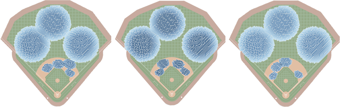
Figure 4. Traditional shift for (a) left-handed and (c) right-handed batters and (b) Standard Positioning.

Our simulations show that an optimal PAP positioning with three infielders lowered predicted BABIP by 5.9% for right-handed batters and by 10.3% for left-handed batters on average when compared with the standard positioning simulation results. The results in Table 1 show the change in BABIP when comparing the traditional shift with the standard positioning (RH/LH BABIP Change) as well as the change in BABIP when comparing the PAP positioning with the standard positioning (PAP BABIP Change). Notice that all batters except Lorenzo Cain see a decrease in BABIP when using the PAP positioning, indicating the batter-specific defensive positioning strategy presented in this work is promising.

Table 1. Percentage change in BABIP after repositioning.

RH Player	RH BABIP Change	PAP BABIP Change	LH Player	LH BABIP Change	PAP BABIP Change
Altuve	0.89%	-7.14%	Freeman	-0.91%	-11.82%
Arenado	4.55%	-6.26%	Bruce	-4.27%	-13.68%
Cain	11.54%	1.92%	Carpenter	-1.80%	-9.91%
Encarnacion	1.79%	-8.39%	Gallo	-2.56%	-5.13%
Frazier	1.79%	-6.25%	Gordon	-1.77%	-9.73%
Longoria	0.00%	-8.93%	Harper	-3.51%	-8.77%
Martinez	4.81%	-3.85%	Heyward	-1.80%	-11.71%
Posey	2.78%	-5.56%	Kiermaier	-0.90%	-9.91%
Pujols	0.90%	-9.91%	Rizzo	-1.80%	-13.51%
Trout	2.68%	-4.46%	Votto	-1.80%	-9.01%

Conclusion

It should be noted that this work includes many simplifying assumptions, but as a proof-of-concept approach to applying binary integer programming techniques to defensive positioning in baseball, the outcome is positive. All situational factors of the game are ignored in this model, meaning that it is run under the assumption that there are no outs and no runners on base. Situational factors like runners on base, the pitch count, the number of outs, the inning, and the score of the game can all impact a coach’s decision on their defensive strategy. It is for this reason that this work can be viewed as a tool that a coach can consider, but is not designed to force positioning decisions. The model is also constructed using averages regarding player speed, both for batters and fielders. As such, this model could become more customizable if individual player elements were included to customize coverage regions. With these enhancements, decision-makers in Major League Baseball may be interested in the findings that this mathematical approach to defensive positioning can bring to a team.

References

Baseball Savant 2019. https://baseballsavant.mlb.com. Accessed on July 26, 2019.