This entry describes some recent results on convergence of equation-free methods from Marschler et al. [2] and Sieber et al [1], and illustrates the results with an example from Quinn et al. [13].

Convergence of equation-free methods for finite time scale separation

The Scholarpedia article [3] by I.G. Kevrekdis and G. Samaey on Equation-free modelling describes a computational approach to implicit model reduction that assumes the existence of a reduced model in a high-dimensional dynamical system without the need to construct an explicit equation for this reduced model. An application area intended for equation-free methodology are multi-particle simulations where particles interact randomly or chaotically, and the reduced model is, for example, some emergent macroscopic low-dimensional system of ordinary differential equations (ODEs). Typical derivations of these reduced models (often called mean field models) make assumptions on closure, replacing higher-order moments or connections by explicit functional expressions of lower-order moments, which the computational equation-free approach avoids.

A didactic random network example. Gross and Kevrekidis [4] use the equation-free methodology to find unstable equililbria of the mean field dynamics for a dynamic random SIS network. The network consists of \(N\) nodes that may be either infected or susceptible. The network is then updated at each time step according to the following rules.

Each infected (I) node recovers with probability \(r\), becoming susceptible (S); along each S-I link, the infection may spead with probablity \(p\), infecting the S node, and each S-I link may be rewired replacing the I vertex by an S node that is not yet connected to the S vertex of the link (avoiding double connections), with probability \(w \rho\), where \(\rho\) is the fraction of I nodes present in the network.

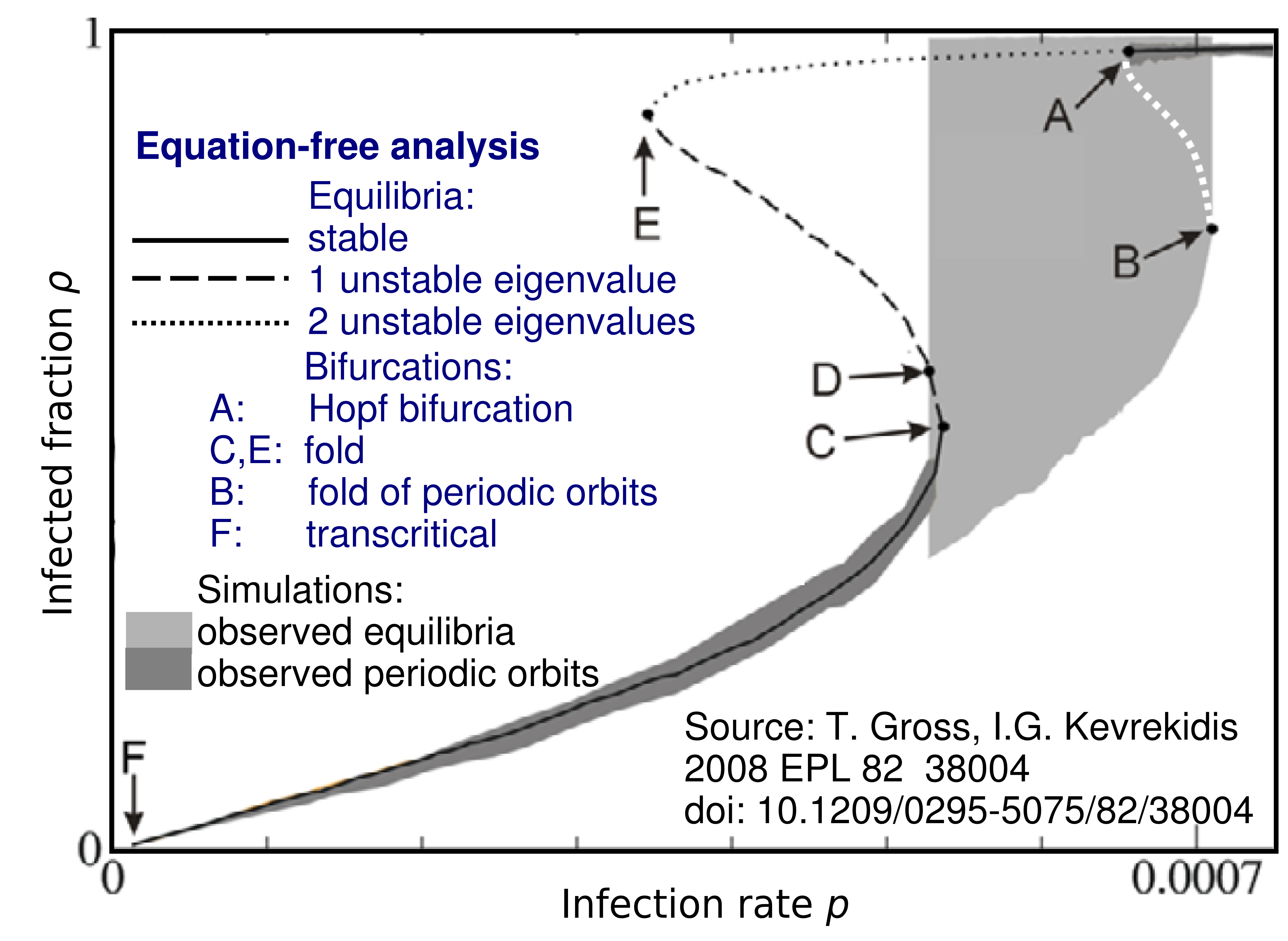
Figure 1. Macroscopic bifurcation analysis using equation-free methods for Gross' random dynamic SIS network. All equilibria and their stability have been computed using the equation-free approach with constraint runs as explained in [7] (not using the implicit formulation (4) explained below). Grey-shaded overlays are results of simulations. White dots are unstable macroscopic periodic orbits hypothesized to be present. At points A, B and C sudden transitions of macroscopic behavior occur. Underlying graph reproduced with permission from iopscience.iop.org, text and legend added.

When all probabilities \(r,p,w\) are small and \(N\) is large then the network shows non-trivial emergent low-dimensional macroscopic dynamics, including a sudden transition to large-amplitude oscillations of the fraction of infected nodes, shown in Figure 1. Gross et al [4] also derive a system of ODEs for the macroscopic dynamics of \(\rho\), \(\ell_{II}\), \(\ell_{SS}\), where, \(\ell_{ab}\) is the density of \(a-b\) links. The derivation of this ODE model assumes that the number of \(a-b-c\) chains is a known function of the number of \(a-b\) and \(b-c\) links and \(b\) nodes. This is a typical closure assumption, which one may avoid with equation-free analysis. Figure 1 shows a-posteriori that the results of the equation-free analysis agree well for stable macroscopic equilibria with the observations from simulations. However, it is unclear whether this holds for unstable equilibria (or periodic orbits), and which concept of convergence is provable.

Illustration for a delay differential equation (DDE). The SIS network is a didactic example of a typical intended scenario for equation-free methods. However, equation-free methodology has originally been formulated and justified for the scenario where the high-dimensional system is deterministic, but has a stable slow manifold \({\cal C}\). We explain the methodology using a deterministic example from Quinn et al. [13] (see [12] for another deterministic example). This demonstration shows how one can apply an algorithm for planar maps to an infinite-dimensional dynamical system defined by a periodically forced DDE, if this DDE has a slow two-dimensional manifold (surface) \({\cal C}\), without deriving an approximate model for the reduced flow on this slow surface. The forced DDE considered in [13] has the form

\(\dot u=-p u(t-\tau)+ru(t)-su(t-\tau)^2-u(t)u(t-\tau)^2-aI(t)\mbox{,}\)

(1)

modeling the Mid-Pleistocene transition (frequency and amplitude of ice age transitions increased markedly about 800,000 years ago). In (1) \(u\) is the non-dimensionalized anomaly in the global ice volume, \(I\) is the fluctuation solar insolation (a multi-frequency quasiperiodic signal), \(\tau\) is the delay caused by ocean overturning and ice response time, and the nonlinearities folllows those for atmoshperic CO\(_2\) in Saltzman and Maasch's models [14]. The parameters are \(r=s=0.8\), \(p=0.95\), \(\tau=1.55\) for the figures below, where time unit is \(10^4\) years. Without forcing the equation has a stable equilibrium and a large amplitude periodic orbit. For forcing \(I(t)\) based on astronomical data and moderate amplitude \(a\in[0.1,0.25]\) the model makes a transition between small amplitude oscillations (a perturbation of the stable equilibrium) and large amplitude oscillations (a perturbation of the large amplitude periodic orbit) at 800,000 years BP, replicating the signal from palaeoclimate records closely [13]. Quinn et al. [13] studied the periodic forcing

\(I(t)=\sin(2\pi t/T)\mbox{,}\)

(2)

where \(T=4.1\) (41,000 years) is the dominant forcing period of the astronomic insolation forcing. For amplitude \(a < 0.3\) one observes that time \(T\)-map \(M^T\) orbits of (1), (2) get attracted to a two-dimensional surface \({\cal C}\), called the slow manifold, shown in (transparent) red in Figure 2.

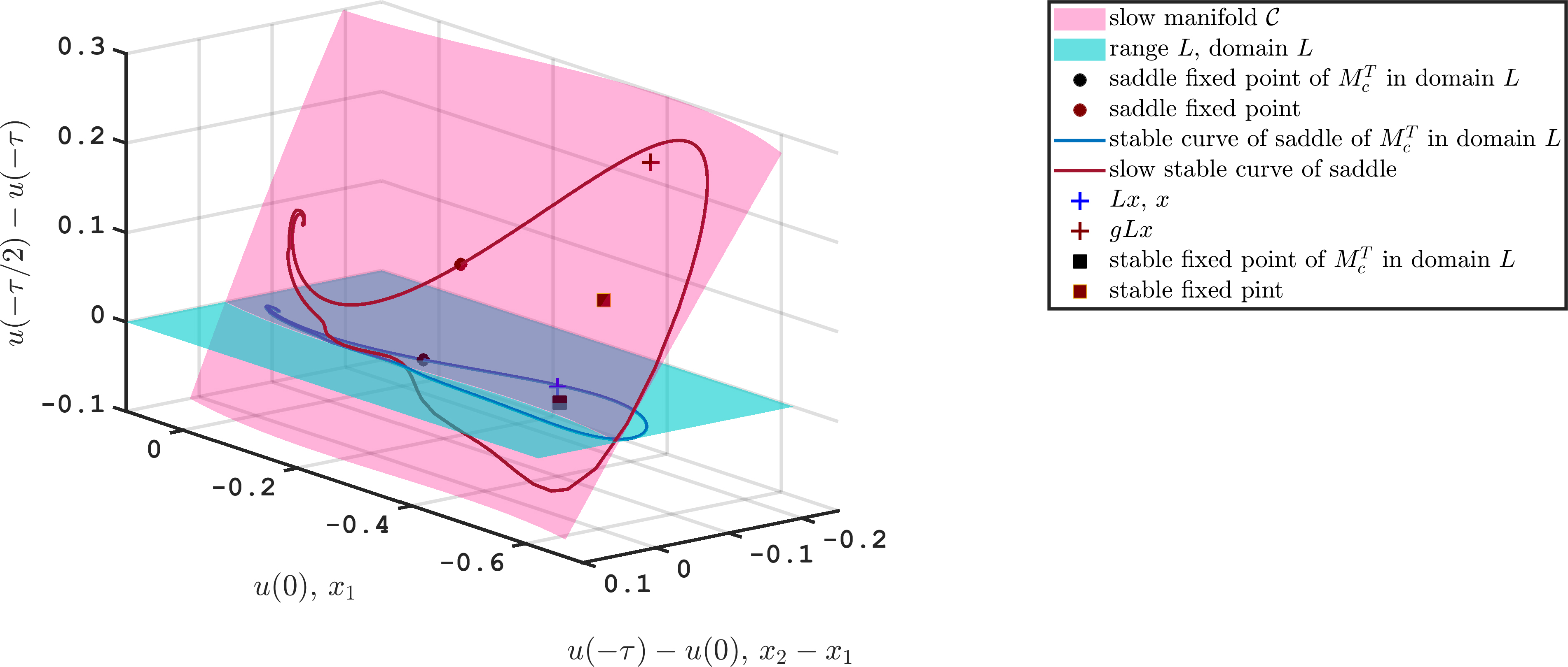
Figure 2. Slow manifold \({\cal C}\) of DDE (1) (dark red transparent surface), saddle and stable fixed point of \(M^T\) (red circle and square) and the intersection between the stable manifold of the saddle and the slow manifold (called slow stable curve in the legend, in red), all in the projection onto \((u(0),u(-\tau)-u(0),u(-\tau/2)-u(\tau))\in\mathbb{R}^3\). The green surface is the projection of the range of the lifting map \(L\) (green surface). In this projection range \(L=\{u:u(-\tau/2)-u(-\tau)=0\}\) is equal to the domain of \(L=\{(x_1,x_2)\) with zero vertical component\(\}\). The black circle and square are the saddle and stable fixed points of the reduced planar map \(M_c^T\) in the coordinates on domain \(L\), and the blue curve is stable curve for the saddle fixed point of \(M_c^T\). The blue cross is a typical point \(Lx\) in range \(L\). The red cross is its image under the stable fiber projection \(g\).

The period-one map \(M^T\) of DDE (1), (2) acts on an infinite-dimensional space \(U\): possible initial values are arbitrary functions \(u\) on \([-\tau,0]\). Figure 2 shows this slow manifold \({\cal C}\) as a surface in the three-dimensional projection onto \((u(0),u(-\tau)-u(0),u(-\tau/2)-u(\tau))\). On the slow manifold \({\cal C}\) the map \(M^T\) is a planar map. The transition scenario for the astronomical forcing is caused by a shift in the basin of attraction of the small-amplitude stable fixed point (shown as red square in Figure 2, corresponding to a periodic orbit of (1), (2)). Hence, the stable curve (red curve) of the saddle fixed point is a boundary of the basin of attraction in the slow manifold, and an object of interest. For planar maps an algorithm for computation of stable curves of saddle fixed points had been proposed and demonstrated by England et al. [15]. The equation-free approach permits us to apply this algorithm directly to the DDE without having to explicitly compute an approximation for the slow manifold. For our DDE case, the user should provide

• a lifting operator, a map \(L\) which maps from \(\mathbb{R}^2\) into \(U\) in the vicinity of the slow manifold \({\cal C}\) (assumed to be of dimension \(2\)); we choose \[L(x_1,x_2):= u:[-\tau,0]\to\mathbb{R}\quad \mbox{where}\quad u(0)=x_1\mbox{,}\quad u(s)=x_2\quad \mbox{for \(s<0\).}\] In the projection of Figure 2 the range of \(L\) is the (transparent green) horizontal plane at vertical component \(u(-\tau/2)-u(-\tau)=0\). The original \(x\) coordinates are are added to the the two horizontal axes such that \(x\) and \(Lx\) have the same coordinates in Figure 2 for all \(x\in\mathbb{R}^2\).
• and a restriction operator, a map \(R\) which maps from \(U\) back into the \(\mathrm{R}^2\); we choose \[Ru=(u(0),u(-\tau))\in\mathbb{R}^2\mbox{.}\]

The DDE map \(M^T\) will transport any initial value \(u\) with some exponential rate \(r_\mathrm{fast}>0\) toward the slow manifold \({\cal C}\) such that \(M^{kT}Lx\) is \(\exp(-r_\mathrm{fast}k)\) close to \({\cal C}\) for \(k\geq1\). Applying the restriction \(R\) to this point on (or close to) the slow manifold \({\cal C}\) projects it back into \(\mathbb{R}^2\) such that the

\[\mbox{lift-evolve-restrict map}\quad P^{kT}x:=RM^{kT}Lx\]

is a map that for each \(k\)-multiple of the forcing period \(T\) maps from the plane \(\mathbb{R}^2\) back into the plane. Equation-free methods in their basic form aim to reconstruct the dynamics on the slow manifold \({\cal C}\) using \(P\).

Exact reduced planar map \(M_c^T\). As part of any claim of reconstruction one needs to specify a coordinate system (or chart) on the manifold \({\cal C}\). Marschler et al [1,2] chose the chart obtained the composition of the lifting map \(L\) with the stable fiber projection \(g:U\to{\cal C}\) onto the manifold \({\cal C}\). This projection \(g\) is defined by the "shadow" \(gu\in{\cal C}\) of a point \(u\in U\), the unique point satisfying

\[M^{kT}u-M^{kT}gu\sim\exp(-r_\mathrm{fast}k)\mbox{ for \(k\to\infty\),}\]

where \(r_\mathrm{fast}\) is the attraction rate toward \({\cal C}\). Thus, \(gu\) is the point in \({\cal C}\) such that \(M^{kT}gu\) tracks \(M^{kT}u\) as closely as possible. Figure 2 shows for a typical point \(Lx\in U\) (blue cross in the green plane) its image \(gLx\in{\cal C}\) under the stable fiber projection \(g\) (red cross in red surface).

A feasibility assumption from [1,2] for equation-free analysis in this simple form is that both maps

\[gL:\mathbb{R}^2\to {\cal C}\mbox{,} \quad \quad \quad R:{\cal C}\to\mathbb{R}^2\]

are (local) diffeomorphisms, that is, the maps have to be invertible between the manifold \({\cal C}\) and the coordinates provided by \(L\) and \(R\) in \(\mathbb{R}^2\). If both assumptions are true then the

\[\mbox{exact reduced planar period-\(T\) map}\quad M^T_c:=(gL)^{-1}\circ M^T\vert_{{\cal C}} \circ gL\mbox{,}\]

on the slow surface \({\cal C}\) in \(gL\) coordinates is given by the implicit expression

\(y_*=M^T_cx\quad \mbox{if \(y_*\) solves} \quad RgLy_*=RM^TgLx\mbox{.}\)

(3)

Since the manifold \({\cal C}\) is and the projection \(g\) are unknown, but \({\cal C}\) is attractive and, hence, \(M^{jT}gL\approx M^{jT}L\) for large integers \(j\), such that we may define the following computable approximation for \(M_c^T\).

Approximate reduced planar map \(M^{j,T}\) and stable fiber projection \(g_j\).

\(M^{j,T}x :=y\quad \mbox{where \(y\) solves \(P^{jT}y=P^{(j+1)T}x\), or, \(RM^{jT}Ly=RM^{(j+1)T}Lx\),}\)

(4)

\(g_jx :=M^{jT}Ly\quad \mbox{where} y \mbox{solves}P^{2jT}y=P^{jT}x\mbox{, or,} RM^{2jT}Ly=RM^{jT}Lx\).

(5)

The additional time \(jT\) that one follows the map \(M\) (of the DDE in our case) in this approximation is called the healing time in review [3]. The stable fiber projections shown in Figure 2 have been computed using the approximation \(g_1\). That is, we have solved \(RM^{2T}Ly=RM^{T}Lx\) and then used \(g_1x=M^TLy\) to plot the red cross. The convergence result in [1] states that

\(M^{j,T}x-M^T_cx \sim \exp(-j(r_\mathrm{fast}-r_\mathrm{slow}))\mbox{,}\)

(6)

\(\partial^kM^{j,T}x-\partial^kM^T_cx \sim \exp(-j(r_\mathrm{fast}-(2k+1)r_\mathrm{slow}))\mbox{,}\)

(7)

where \(r_\mathrm{slow}\) is the maximal rate of attraction or expansion along the tangential (slow) direction of the slow manifold \({\cal C}\).

Planar stable curve algorithm by England et al. [15] for \(M^{1,T}\). The (unknown) exact map \(M_c^T\) and the approximate map \(M^{j,T}\) are both maps in \(\mathbb{R}^2\). We can now determine the stable curves of a saddle fixed point (which is a saddle periodic orbit of the DDE (1)) for the map \(M^{1,T}\) using the algorithm from [15] for this implicitly defined map. The algorithm grows the curve from the saddle backward by finding pre-images of curves without Newton iteration.

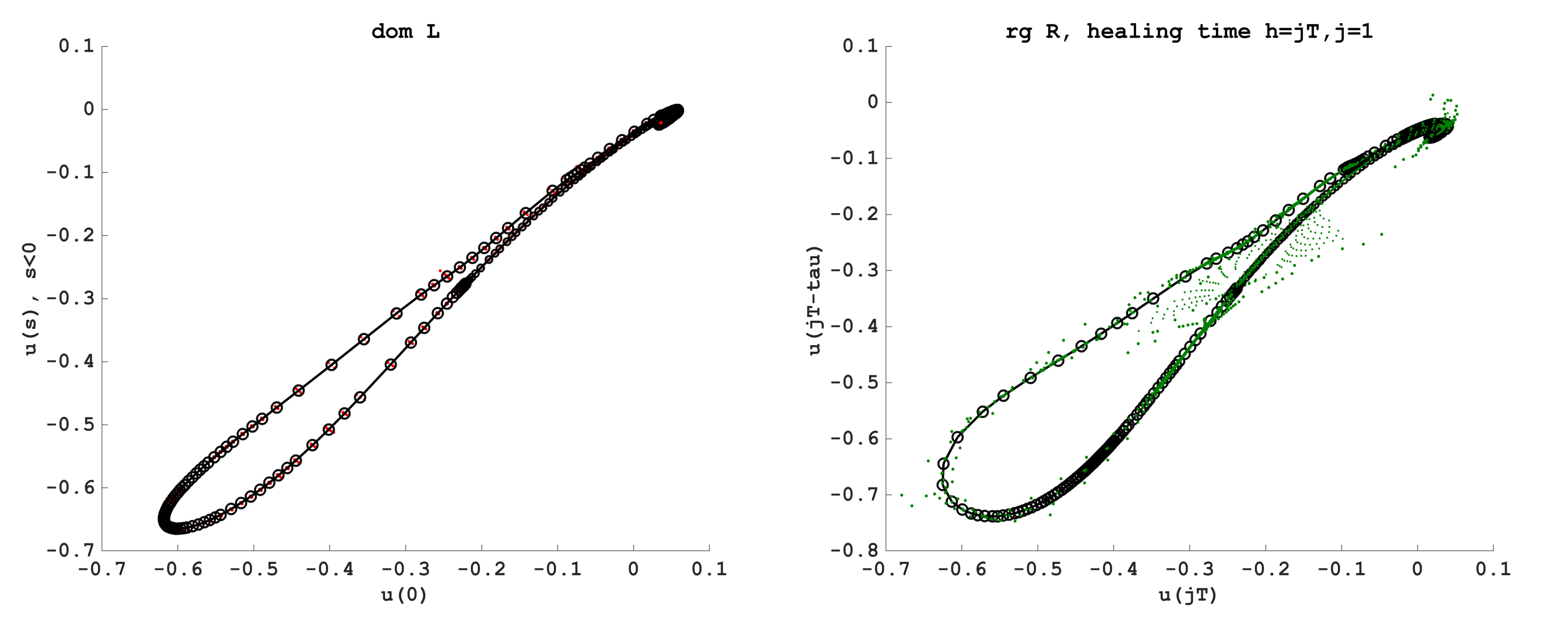
Figure 3. Output of stable curve algorithm for non-invertible maps in the coordinates of the domain of \(L\) for the map \(M^{1,T}\approx M_c^T\) (left) and in the coordinates of range \(R\) (right). the circles show the adaptive computational steps taken by the algorithm the colored dots show the test points used during a circle bisection during each step.

The algorithm's final state is shown in Figure 3, where the adaptive stepsize is visible. An animation of the manifold growth is shown in Figure 5 and downloadable from D1. A didactic implementation in Matlab/octave compatible code is downloadable from D2. The original code was modified to avoid solving the equation defining \(M^{1,T}\) at every step.

Continuous time semiflows. For continuous time flows \(M^t:\mathbb{R}^D\to\mathbb{R}^D\) with large \(D\) and \(t\in[0,\infty)\) the construction of the approximate slow flow \(M^{h,t}\) and stable fiber projection \(g_h\) with healing time \(h\geq0\) are (assuming that the slow manifold is \(d\) dimensional with \(d < D\))

\[M^{h,t}x:=y\quad \mbox{where \(y\) is the solution of \(RM^hLy=RM^{t+h}Lx\),}\] \[g_hx:=M^hLy\quad \mbox{where \(y\) is the solution of \(RM^{2h}Ly=RM^hLx\),} \mbox{.}\]

which satisfy [1]

\(M^{h,t}x-M^t_cx \sim \exp(-h(r_\mathrm{fast}-r_\mathrm{slow}))\mbox{,}\)

(8)

\(\partial^kM^{h,t}x-\partial^kM^t_cx \sim \exp(-h(r_\mathrm{fast}-(2k+1)r_\mathrm{slow}))\mbox{.}\)

(9)

Figure 4 illustrates how choosing longer healing time improves accuracy of the approximation in this idealized scenario. In this illustration the high-dimensional space is compressed into the plane, the slow manifold \({\cal C}\) (green) is horizontal, with motion on the slow manifold uniformly slowly to the left, the lifting \(L\) is onto the horizontal line above \({\cal C}\), and the restriction \(R\) is the projection down onto the horizontal axis. Attraction toward the slow manifold is vertical such that any initial conditions lying on the same yellow line (stable fiber) have the same forward limit, so they have the same projection \(g\).

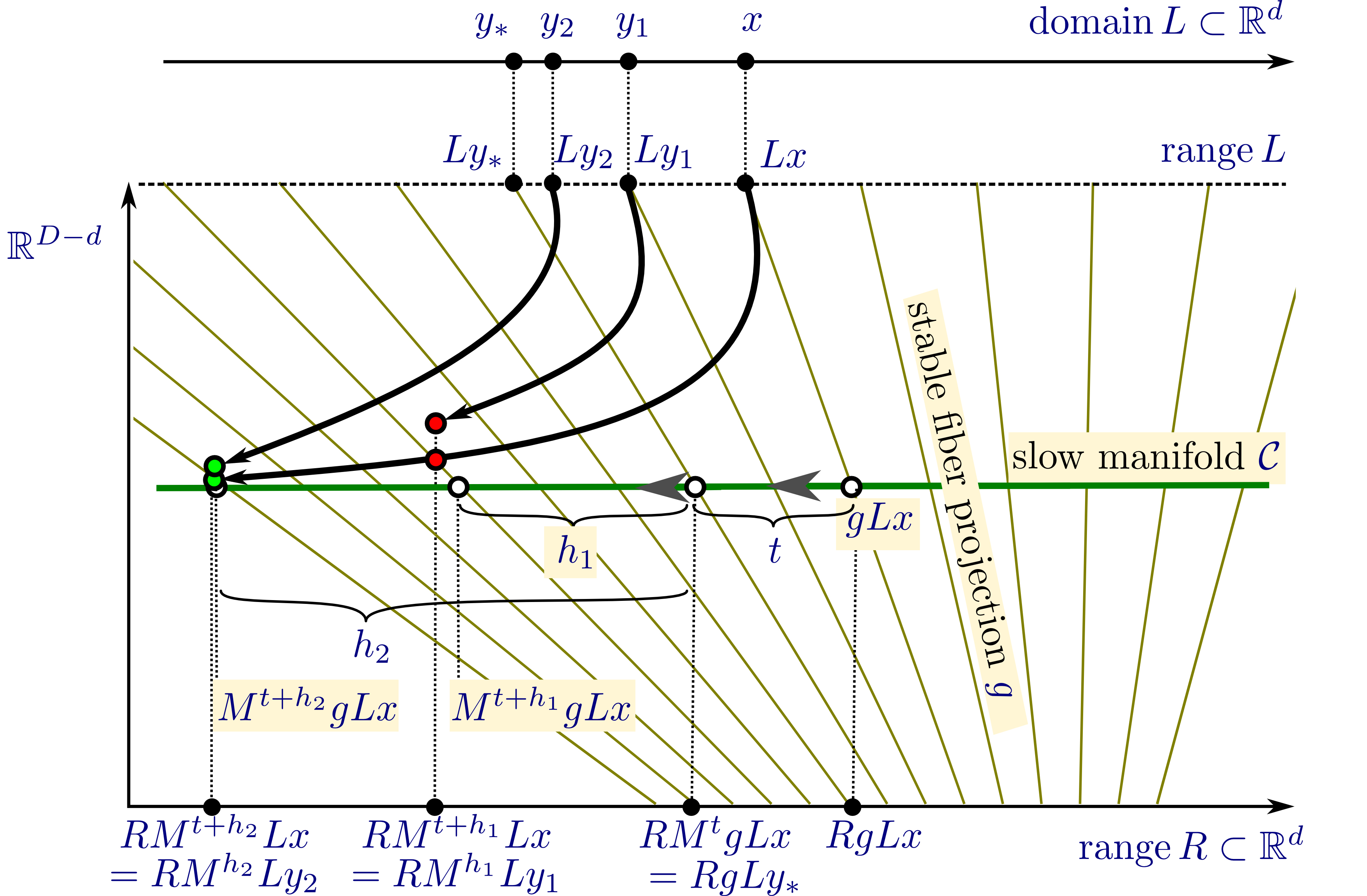
Figure 4. Illustration of approximation of reduced flow \(M^t_c\) by approximate flow \(M^{h,t}\) for two different healing times \(h_1\) and \(h_2\). The exact reduced flow is \(y_*=M^t_cx\) (where \(y_*\) is defined by \(RgLy_*=RM^tgLx\)). The yellow lines are the stable fibers. They provide the coordinate chart for the flow on \({\cal C}\) in the range of \(L\)). The result of the approximate reduced flow \(M^{h_1,t}\) is defined by requiring that the red dots (\(M^{t+h_1}Lx\) and \(M^{h_1}Ly_1\)) have the same projection horizontally (same for \(h_2\)). Convergence implies that the green dots are closer to the corresponding white dot \(M^{t+h_2}gLx\) on \({\cal C}\) than the red dots to their corresponding white dot \(M^{t+h_1}gLx\).

Limitations for finite accuracy. The theoretical result in (6) and (7) suggests that choosing the healing time \(h\) larger improves the accuracy of the result. In practice this effect is limited by the non-zero error \(\Delta\) that occurs when one evaluates \(L\), \(R\) or \(M^t\). Thus, we get the optimal practical values for \(h\) and the resulting overall error \(e\) according to [1]

\(h \sim\frac{-\log\Delta}{r_{\mbox{slow},+}+r_\mbox{fast}}\)

(10)

\(e \sim \Delta^p\quad \mbox{where}\quad p=\frac{r_\mathrm{fast}-r_{\mathrm{slow},-}}{r_\mathrm{fast}+r_{\mathrm{slow},+}}\mbox{.}\)

(11)

In these estimates we distinguish between the expansion rates forward in time, \(r_{\mathrm{slow},+}\), and backward time, \(r_{\mathrm{slow},-}\) tangential to the slow manifold. The previously used quantity \(r_\mathrm{slow}\) is the maximum of \(|r_{\mathrm{slow},-}|\) and \(|r_{\mathrm{slow},+}|\).

The above estimates hold for the equation-free framework in its basic form, where lifting and restriction are a-priori chosen, satisfying a genericity condition. Recent advances demonstrate how one may automatically adjust the dimension of the slow manifold [11] and the range of the lifting \(L\) using diffusion maps.

Discussion for stochastic systems. Sieber et al. [1] give two further demonstrations: the first is a deterministic two-dimensional slow-fast system for Michaelis-Menten kinetics (in rotated coordinates, also used in [7]), which illustrates the convergence rates for fixed time scale separation \(r_\mathrm{slow}/r_\mathrm{fast}\) and increasing healing time \(h\).

The second demonstration follows the analysis by Barkley et al. [8] of a one-dimensional stochastic differential equation (simulating a particle without inertia in a double well potential subject to white noise). The underlying time scale separation occurs in the Fokker-Planck equation (FPE) for the distributions of ensemble simulations. In contrast to the moment maps based directly on the lift-evolve-restrict map \(P^t\) (without healing, see [8] for analysis), the reduced map \(M^{h,t}\) is approximately linear, as is the original FPE. However, the trade-offs caused by low precision of ensemble computations become visible, leading to small optimal values for healing time \(h\), according to (10), and large errors \(e\), according to (11). Noise reduction for ensemble computations may be possible to avoid problems for basic nonlinear algorithms relying on derivative information (such as Newton iterations) [10].

The discussion in [1] points out that in many cases (such as the didactic network example) the goal of equation-free analysis may not be a dimension reduction for the (linear) FPE, but rather a stochastic model reduction, a reduction from a high-dimensional stochastic model to a low-dimensional stochastic model (see review by Givon et al. [9]) without explicit model derivation. For equation-free stochastic model reduction based on the results in [9] convergence results for finite time scale separation are unlikely to hold (at least not using the arguments in [1]), since the stable fiber projection \(g\) does not exist.

Figure 5. Animation of stable-curve algorithm by J. P. England, B. Krauskopf, and H. M. Osinga, adapted for implicit maps.

Acknowledgements. J.S. gratefully acknowledges the financial support of the EPSRC via grants EP/N023544/1 and EP/N014391/1, and from the European Union's Horizon 2020 Research and Innovation Programme under the Marie Sklodowska-Curie grant agreement No 643073. 

Downloadable files

1. Animation of stable-curve algorithm by England et al. [15], adapted for implicit maps dde-stable-mf-growth.mp4.
2. Demonstration code for stable-curve algorithm by England et al. [15], adapted for implicit maps from supplementary material to [13], doi: 10.6084/m9.figshare.7048292.v1, then download matlabdemo.zip.

References

[1]   J. Sieber, C. Marschler, and J. Starke, Convergence of equation-free methods in the case of finite time scale separation with application to stochastic systems, J. Appl. Dyn. Syst., 17 (2018), pp. 2574--2614, doi: 10.1137/17M1126084, arxiv: 1701.08999.

[2]   C. Marschler, J. Sieber, R. Berkemer, A. Kawamoto, and J. Starke, Implicit Methods for Equation-Free Analysis: Convergence Results and Analysis of Emergent Waves in Microscopic Traffic Models, J. Appl. Dyn. Syst., 13 (2014), pp. 1202--1238, doi: 10.1137/130913961, arxiv: 1301.6044.

[3]   I. G. Kevrekidis and G. Samaey, Equation-free modeling, Scholarpedia, 5 (2010), p. 4847, www.scholarpedia.org/article/Equation-free_modeling.

[4]   T. Gross and I. G. Kevrekidis, Robust oscillations in SIS epidemics on adaptive networks: Coarse graining by automated moment closure, EPL (Europhysics Letters), 82 (2008), p. 38004, doi: 10.1209/0295-5075/82/38004, arxiv: nlin/0702047.

[5]   N. Fenichel, Geometric singular perturbation theory for ordinary differential equations, Journal of Differential Equations, 31 (1979), pp. 53--98, doi: 10.1016/0022-0396(79)90152-9.

[6]   M. Hirsch, C. Pugh, and M. Shub, Invariant Manifolds, vol. 583 of Lecture Notes in Mathematics, Springer-Verlag, Berlin, 1977.

[7]   C. W. Gear, T. J. Kaper, I. G. Kevrekidis, and A. Zagaris, Projecting to a slow manifold: Singularly perturbed systems and legacy codes, J. Appl. Dyn. Syst., 4 (2005), pp. 711--732, doi: 10.1137/040608295, arxiv: physics/0405074.

[8]   D. Barkley, I. G. Kevrikidis, and A. M. Stuart, The moment map: nonlinear dynamics of density evolution via a few moments, J. Appl. Dyn. Syst., 5 (2006), pp. 403--434, doi: 10.1137/050638667, arxiv: cond-mat/0508551.

[9]   D. Givon, R. Kupferman, and A. Stuart, Extracting macroscopic dynamics: model problems and algorithms, Nonlinearity, 17 (2004), p. R55, doi: 10.1088/0951-7715/17/6/R01, citeseerx.ist.psu.edu.

[10]   D. Avitabile, R. Hoyle, and G. Samaey, Noise reduction in coarse bifurcation analysis of stochastic agent-based models: an example of consumer lock-in, J. Appl. Dyn. Syst., 13 (2014), pp. 1583--1619, doi: 10.1137/140962188, arxiv: 1403.5959.

[11]   R. R. Coifman, I. G. Kevrekidis, S. Lafon, M. Maggioni, and B. Nadler, Diffusion maps, reduction coordinates, and low dimensional representation of stochastic systems, Multiscale Modeling & Simulation, 7 (2008), pp. 842--864, doi: 10.1137/070696325, pdfs.semanticscholar.org.

[12]   A. Ben-Tal and I. G. Kevrekidis, Coarse-graining and simplification of the dynamics seen in bursting neurons, J. Appl. Dyn. Syst., 15 (2016), pp. 1193--1226, doi: 10.1137/151004574.

[13]   C. Quinn, J. Sieber, and A. von der Heydt, Effects of periodic forcing on a Paleoclimate delay model, preprint, 2019, arxiv: 1808.02310.

[14]   B. Saltzman and K. A. Maasch, Carbon cycle instability as a cause of the late pleistocene ice age oscillations: modeling the asymmetric response, Global biogeochemical cycles, 2 (1988), pp. 177--185, doi: 10.1029/GB002i002p00177.

[15]   J. P. England, B. Krauskopf, and H. M. Osinga, Computing one-dimensional stable manifolds and stable sets of planar maps without the inverse, J. Appl. Dyn. Syst., 3 (2004), pp. 161--190, doi: 10.1137/030600131.