In this entry E. Siero describes some work on dryland vegetation patterns, with excerpts from [12] and [14].

Self-organisation into spatial patterns can play an important role in system functioning. Here we view the dynamics of vegetation patterns in drylands: a very active and relevant field in ecology due to its role in combating desertification. Patterns are viewed as precursors of a catastrophic transition to the degraded bare desert state.

Various low-dimensional (phenomenological) models have been proposed to help explain desertification and vegetation patterns. A prominent example is the Klausmeier model [7], where a surface water component interacts with the vegetation component. This model and variants thereof have been studied extensively since then, see e.g. [11,17,18], and are still being studied, as demonstrated by recent work presented at the NWCS18 conference [1-3,5,9,13].

We now introduce (a variant of) the Klausmeier model. Although rainfall can change seasonally and tends to be intermittent in time, here we view rainfall as a climatic parameter that may slowly change over time and is constant in the absence of climate change. The water evaporation is modeled by a linear term. The positive infiltration feedback makes the uptake terms positively depend on the amount of vegetation. Here we assume they are of the form \(\pm wn^2\), a mass action law with linear positive infiltration feedback. Plant death is, for simplicity, modeled by a linear term. The isotropic spread of water and vegetation is modeled by diffusion terms. Additionally we allow for terrain having a constant slope: downslope advection of water is modeled by \(vw_x\). Together this gives
\begin{equation*} \label{eq:extK2D}
 \begin{alignedat}{3}
  w_t=&d\Delta w+vw_x&+a(t)-w-wn^2, \\
  n_t=&\Delta n&-mn+wn^2,
 \end{alignedat}
\end{equation*} with \(\Delta=\frac{\partial^2}{\partial x^2}+\frac{\partial^2}{\partial y^2}\). Because vegetation patterns extend over large areas, the spatial domain is taken to be \(\mathbb{R}^2\), so without boundary conditions. Regularly used parameters are \(m=0.45\) and \(d=500\), where \(d\gg 1\) since water spreads faster than vegetation.

As a consequence of climate change, rainfall \(a(t)\) in drylands is expected to decrease as a function of time. The model has a homogeneously vegetated steady state of inhibitor-activator type, which becomes Turing(-Hopf) unstable as rainfall \(a\) gets below a critical value. Beyond the instability a set of stable striped patterns exists (perpendicular to the advection, for \(v>0\)), whose wavenumbers form an interval. In Figure 1 a simulation is shown, for advection \(v=365\) with \(\frac{da}{dt}=10^{-5}\), where pattern formation occurs between \(a=4.5\) and \(a=4.4\). During the further decrease of \(a\) the striped pattern coarsens a few times (decreasing number of stripes), before transverse instabilities take hold. Eventually, for sufficiently small rainfall, the bare desert state is reached.

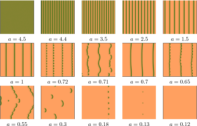
Figure 1: Frames from a simulation with slowly decreasing parameter \(a\), \(da/dt=-10^{-5}\), for \(v=365\), (\(d=500\) and \(m=0.45\)) with periodic boundary conditions. Gradient ranging from \(n=0\) (sandy-brown) to \(n=21.45\) (dark-green). Initial condition just before the Turing-Hopf bifurcation (\(a=4.5\)). After that, consecutive striped patterns with decreasing number of stripes, before stripes break up a first time at \(a=0.72\). Newly formed stripes break up again at \(0.65\), followed by dynamics in 2D and eventually a bare desert state. Domain size \(250\times 250\).

 

An overview of observable striped vegetation can be computed using continuation software [4,16]. The graphical representation of this overview is referred to as the Busse balloon (of striped patterns). A transition occurs when a changing parameter drives the system outside the Busse balloon. Knowledge of Busse balloons thus adds predictability to complex system dynamics.

To determine spectral stability of a striped pattern \((\bar w,\bar n)\) with wavenumber \(\kappa\),
\begin{equation*}
 (\bar w,\bar n)(x)=(\bar w,\bar n)\left(x+\frac{2\pi}{\kappa}\right),
\end{equation*} we linearize. Combining Floquet-Bloch decomposition in the \(x\)-direction and Fourier transform in the \(y\)-direction, 2D perturbations \((W,N)\) are decomposed in products \(N_\gamma (x)e^{\mathrm{i}\ell y}\) that satisfy
 \begin{equation*}
   N_\gamma\left(x+\frac{2\pi}{\kappa}\right)e^{\mathrm{i}\ell y}=\gamma N_\gamma(x)e^{\mathrm{i}\ell y}
 \end{equation*} with \(\gamma\in S^1\subset\mathbb{C}\) and \(\ell\in\mathbb{R}\) (and similarly for \(W\)).

We are now interested in situations where \(\Re(\lambda(\gamma,\ell))\approx 0\). Restriction to perturbations with \(\ell=0\) corresponds to stability of patterns in the 1D model (where the \(y\)-coordinate is removed). Perturbations with \(\ell\neq 0\) are not constant in the transverse \(y\)-direction along the stripes and may cause them to break up. Numerical study indicates that the most relevant instabilities are: 
Sideband. Case where \(\ell=0\), \(\gamma\approx 1\) (1D). By translation invariance, there is always a neutrally stable eigenvalue \(\lambda(1,0)=0\). Since \(\Re(\lambda(\gamma,\ell))\) is invariant with respect to complex conjugation of \(\gamma\), this leads to genericity of an instability where the curve \(\Re(\lambda(\gamma,0))\) changes from concave to convex. Constraint: 
\begin{equation*}
 \frac{\partial^2}{\partial\gamma^2}\Re(\lambda(\gamma,0))=0 \text{ at } \gamma=1
\end{equation*}
Stripe-rectangle breakup. Case where \(\ell\neq 0\), \(\gamma=1\) (2D). Transverse destabilization with same phase in neighboring stripes. Constraint:
\begin{equation*} 
 \Re(\lambda(1,\ell))=\frac{\partial}{\partial \ell}\Re(\lambda(1,\ell))=0
\end{equation*}
Stripe-rhomb breakup. Case where \(\ell\neq 0\), \(\gamma=-1\) (2D). Transverse destabilization with opposite phase in neighboring stripes. Constraint:
\begin{equation*} 
 \Re(\lambda(-1,\ell))=\frac{\partial}{\partial \ell}\Re(\lambda(-1,\ell))=0
\end{equation*} Tracing marginal stability by continuation under one of these constraints, forms the basis of the computation of the Busse balloons in Figure 2.

When during a simulation the system resides in a striped pattern it can be represented by a single wavenumber. These wavenumbers are compared with the corresponding Busse balloon in Figure 2. For decreasing rainfall \(a\), the system first hits the 1D black sideband instability, leading to replacement of one striped pattern by another. For smaller \(a\), the system hits the breakup instabilities first, as the striped pattern is replaced by a pattern of spots.

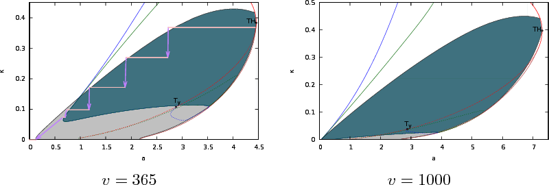
Figure 2: Busse balloon of stable striped patterns for \(v=365\) and \(v=1000\) (with \(d=500\) and \(m=0.45\)). The union of all colored regions bounded by the black sideband curve represents striped patterns that are 1D stable. The blue and green curve indicate marginal stability against stripe-rectangle and stripe-rhomb breakup respectively. Full 2D stability is indicated by the dark-green (teal) color. In the Busse balloon on the left, the wavenumber during the simulation of Figure 1 is indicated with pink if the system resides in a striped pattern state, purple arrows in between indicate transient dynamics or residence in 2D states before returning to a striped pattern (or the bare desert state \(\kappa=0\)). In the Busse balloon on the right, most of the 1D stable patterns are also stable in 2D, even extending partly to large wavelengths: \(\kappa=0\).

The extent to which striped patterns are susceptible to breakup, depends on the slope. On flat ground (\(v=0\)), all large wavelength (`pulses', small wavenumber \(\kappa\)) patterns are transversely unstable. In Figure 3 the Busse balloon of stable striped patterns is also plotted for \(v=1000\), in this case almost all striped patterns that are stable in 1D are also transversely stable. For recent work on (transverse) stability of large wavelength patterns with large advection, see [1,3,8,10].

The agreement between stable striped patterns in the Busse balloons and observed striped patterns in the simulations with a changing parameter (i.e. \(\frac{da}{dt}=-10^{-5}\)), is closer if the rate of change is small: the length of trajectories outside the Busse balloon and the jumps in wavenumber get larger if the rate of change increases [15]. In this movie (again with domain \(250\times 250\) and periodic boundary conditions), the rate of change (\(\frac{da}{dt}=-10^{-2}\)) is too large for convergence to a steady state and no clear jump from one striped pattern to another is visible. Note that the vegetation is actually moving uphill. In a study of patterns in Somalia it was found that in areas where bands have not completely disappeared, changes in wavelength are imperceptible [6]. One possible reason for this could be that conditions either changed too fast, or barely changed at all.

 

References

[1] R. Bastiaansen, P. Carter and A. Doelman, Stable planar vegetation stripe patterns on sloped terrain in dryland ecosystems, In preparation.

[2] R. Bastiaansen, O. Jaïbi, V. Deblauwe, M.B. Eppinga, K. Siteur, E. Siero, S. Mermoz, A. Bouvet, A. Doelman and M. Rietkerk, Multi-stability of model and real dryland ecosystems through spatial self-organization, Preprint.

[3] P. Carter and A. Doelman, Traveling stripes in the Klausmeier model of vegetation pattern formation, Preprint.

[4] E.J. Doedel, T.F. Fairgrieve, B. Sandstede, A.R. Champneys, Y.A. Kuznetsov and X. Wang, Continuation and bifurcation software for ordinary differential equations, Technical report, 2007, http://cmvl.cs.concordia.ca/auto.

[5] P. Gandhi, L. Werner, S. Iams, K. Gowda and M. Silber, A topographic mechanism for arcing of dryland vegetation bands, Preprint.

[6] K. Gowda, S. Iams and M. Silber, Signatures of human impact on self-organized vegetation in the Horn of Africa, Scientific Reports, 8(1), 2018.

[7] C.A. Klausmeier, Regular and irregular patterns in semi-arid vegetation, Science, 284:1826--1828, 1999.

[8] T. Kolokolnikov, M. Ward, J.C. Tzou and J. Wei, Stabilizing a homoclinic stripe, Preprint.

[9] R. Samuelson, Z. Singer, J. Weinburd and A. Scheel, Advection and autocatalysis as organizing principles for banded vegetation patterns, Journal of Nonlinear Science, 2018.

[10] L. Sewalt and A. Doelman, Spatially periodic multipulse patterns in a generalized Klausmeier-Gray-Scott model, SIAM Journal on Applied Dynamical Systems, 16(2):1113--1163, 2017.

[11] J.A. Sherratt, Using wavelength and slope to infer the historical origin of semiarid vegetation bands, Proceedings of the National Academy of Sciences, 112(14):4202--4207, 2015.

[12] E. Siero, A recipe for desert: Analysis of an extended Klausmeier model, PhD thesis, Leiden University, 2016.

[13] E. Siero, Nonlocal grazing in patterned ecosystems, Journal of Theoretical Biology, 436:64--71, 2018.

[14] E. Siero, A. Doelman, M.B. Eppinga, J.D.M. Rademacher, M. Rietkerk and K. Siteur, Striped pattern selection by advective reaction-diffusion systems: Resilience of banded vegetation on slopes, Chaos: An Interdisciplinary Journal of Nonlinear Science, 25, 2015.

[15] K. Siteur, E. Siero, M.B. Eppinga, J.D.M. Rademacher, A. Doelman and M. Rietkerk, Beyond Turing: the response of patterned ecosystems to environmental change, Ecological Complexity, 20:81--96, 2014.

[16] H. Uecker, D. Wetzel, and J.D.M. Rademacher, pde2path - A Matlab package for continuation and bifurcation in 2D elliptic systems, Num. Math.: Th. Meth. Appl., 7:58--106, 2014.

[17] S. van der Stelt, A. Doelman, G. Hek and J.D.M. Rademacher, Rise and fall of periodic patterns for a Generalized Klausmeier-Gray-Scott model, J. Nonl. Sc., 23:39--95, 2013.

[18] J. von Hardenberg, E. Meron, M. Shachak and Y. Zarmi, Diversity of Vegetation Patterns and Desertification, Physical Review Letters, 87:3--6, 2001.