(1)\begin{align}
\dot x &= \frac{1}{2} \mu y - (1+\mu) z ,\\
\dot y &= 1 ,\\
\varepsilon \dot z &= x + z^2 .
\end{align}
The parameter \( \mu \) determines the type of folded singularity; \( \mu < 0 \) corresponds to a folded saddle, \( \mu > 0 \) to a folded node.
We note that a simple coordinate transformation of this system results in a system which is no longer singularly perturbed and corresponds to the rescaling chart within a point blow-up analysis.
(2)\begin{align}
\dot x &= \frac{1}{2} \mu y - (1+\mu) z ,\\
\dot y &= 1 ,\\
\dot z &= x + z^2 .
\end{align}
There are two known algebraic solutions of this system which correspond to the singular true and faux canards, respectively,
(3)\begin{align}
\gamma_t &= \Big( -\frac{1}{4} t^2 + \frac{1}{2}, t, \frac{1}{2} t \Big) ,\\
\gamma_f &= \Big( -\frac{1}{4} \mu^2 t^2 + \frac{1}{2} \mu, t, \frac{1}{2} \mu t \Big) .
\end{align}
Recent work by Vo and Wechselberger [3] suggest that there may be rotational behaviour near the folded saddle. To investigate we study the variation equation of (2) about \( \gamma_t \) and \( \gamma_f \). While there is no rotational behaviour near \( \gamma_t \), trajectories near \( \gamma_f \) may indeed rotate about \( \gamma_f \) where the number of rotations is \( \mu \)-dependent.
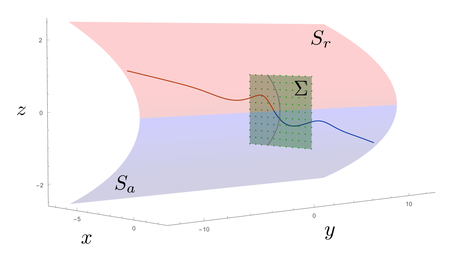
Figure 2: Numerically obtaining the two-parameter family of faux canards. Choosing a section \( \Sigma = \{ y=0 \} \) which is transverse to the flow we can locate faux canard solutions as trajectories which converge to the attracting sheet of the critical manifold in forward time and the repelling sheet of the critical manifold in backward time. This method of calculating faux canards is numerically stable, unlike a shooting method from either sheet of the critical manifold.
We then proceed to investigate the two parameter family of faux canards guaranteed to exist in (1) and thus also in (2). We first develop a stable scheme by which we may obtain the entire two parameter family of faux canards, shown in figure 2. The attracting and repelling sheets of the critical manifold about the folded saddle are shown in blue and red, respectively. We choose a section transverse to the flow,
(4)\begin{equation}
\Sigma = \{ (x,y,z) \; \vert \; y=0 \} ,
\end{equation}
shown in green. We then take a uniform mesh of points within this section and then flow forward and backward in time to stably calculate solution trajectories near the folded saddle. Solutions either approach the critical manifold near \( \gamma_f \) or else they diverge from the critical manifold. Faux canard solutions are those which approach the critical manifold in both forward and backward in time.
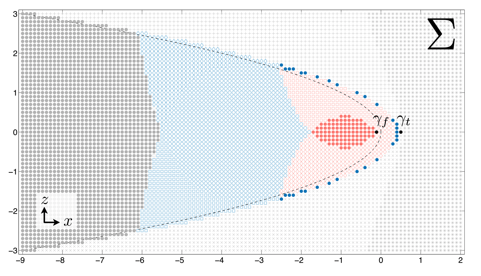
Figure 3: Sectors of solutions within \( \Sigma \) according to rotation number. An array of initial conditions within \( \Sigma \) for \( \mu = -0.22 \) is shown in (x, z)-space. Each initial condition is colored according to the rotation number of the corresponding solution trajectory; 0 (grey), 1 (blue), 2 (orange). The behavior of each trajectory as \( t \rightarrow \pm \infty \) is determined in relation to \( \gamma_f \), i.e., as being on one side or the other of \( \gamma_f \) in a projection onto (y,z)-space. The various combinations are indicated by an open circle (L/R), closed circle (R/L), diamond (L/L), or square (R/R), where L and R denote the side of \( \gamma_f \) to which a trajectory lies in (y,z)-space, first for \( t \rightarrow - \infty \) and then for \( t \rightarrow + \infty \). Diverging trajectories are indicated in one of three ways: by + for those which diverge for \( t > 0 \), by × for those which diverge for \(t < 0\), and by ∗ for those which diverge for both \( t < 0 \) and \( t > 0 \). The intersections of γ1 and γ2 with Σ are indicated in black. The parabola \( x + z^2 = 0 \) is included (black, dashed) for comparison.
We then classify all solutions according to (i) number of rotations about \( \gamma_f \) and (ii) limiting behaviour as \( t \rightarrow \pm \infty \) in relation to \( \gamma_f \) (i.e., lying to the left or right of \( \gamma_f \) at each terminus). As all other solutions are classified in relation to \( \gamma_f \) we term \( \gamma_f \) the primary faux canard. Each solution passing through \( \Sigma \) is then assigned a symbol denoting terminal behaviour and a colour denoting rotation number about the primary faux canard. If these coloured symbols are plotted within \( \Sigma \) at the point of intersection with the corresponding solution we obtain a diagram like that shown in figure 3.
Note the concentric pattern of faux canards surrounding the primary faux canard with highest rotation number near the centre. Also note that grouping solutions according to terminal behaviour indicates sets of solutions (or sectors) with similar behaviour. These sectors also seem to admit continuous boundaries which give rise to the intricate pattern of different solutions.
We reason that the boundary between solutions which converge to the attracting (repelling) sheet of the critical manifold and those which diverge is the attracting (repelling) slow manifold. These manifolds intersect along \( \gamma_t \). By considering the arrangement of faux canards we also reason that the the boundaries which organise the two parameter family of faux canards are the (nonlinear) stable and unstable fiber bundles, which are termed the repelling and attracting fast manifolds, respectively.
Using a 2 point boundary value problem (BVP) we are able to numerically obtain both slow and fast manifolds. The key point is that the calculation of slow manifolds requires a horizontal continuation of one endpoint of the BVP along the critical manifold, approximating the nonlinear tangent bundle of the slow manifold. On the other hand the calculation of fast manifolds requires a vertical continuation of one endpoint of the BVP off the critical manifold approximating the nonlinear fibre bundle of the fast manifold.
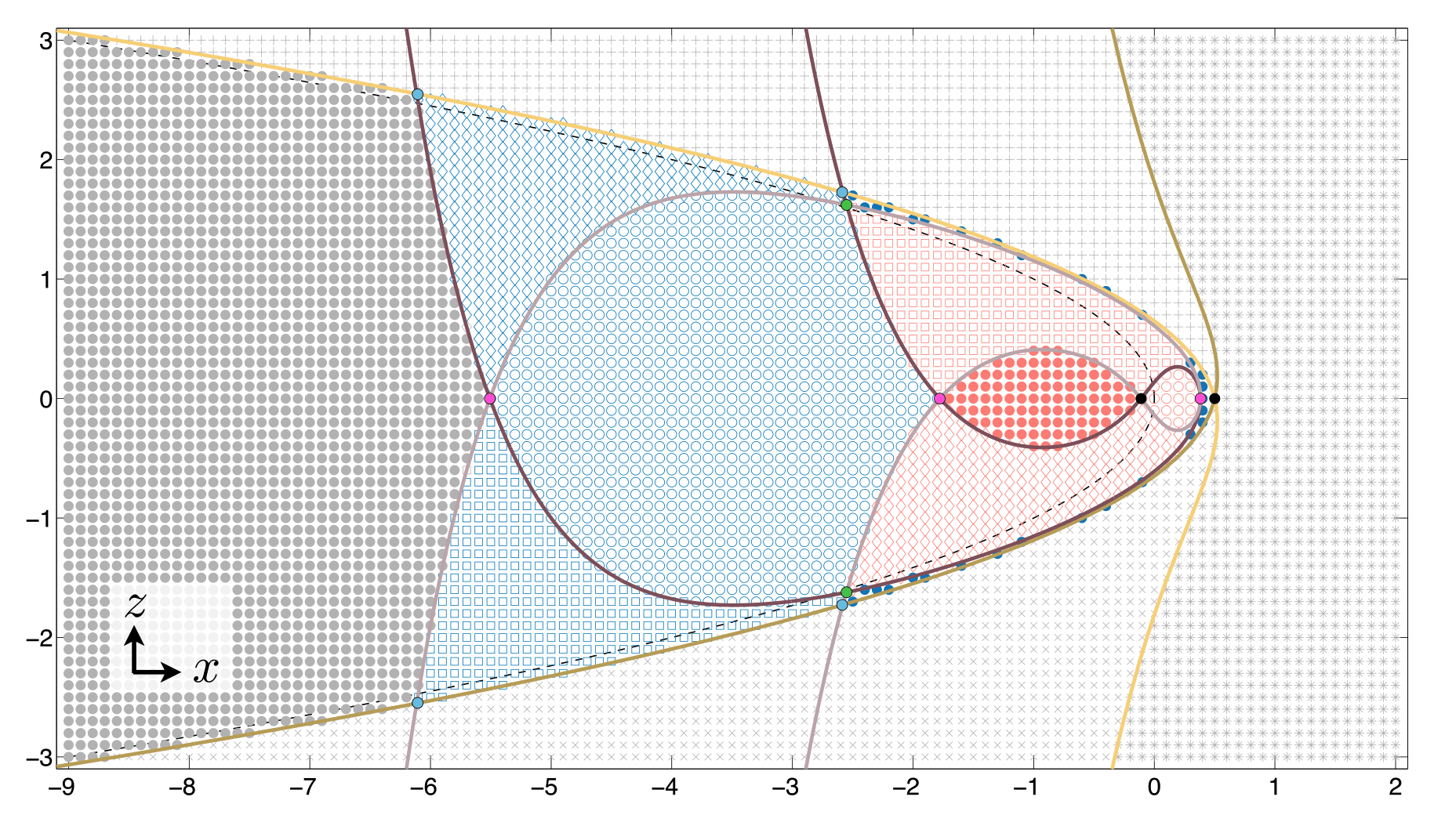
Figure 4: Boundary curves of rotation sectors. Figure 3 with the intersection of fast manifolds (purple) and slow manifolds (gold). The sole intersection between slow manifolds corresponds to \( \gamma_t \). The intersections between fast manifolds are indicated in pink, green, and black corresponding to secondary \( \alpha \)-faux canards, secondary \( \beta \)-faux canards, and \( \gamma_f \), respectively. The intersections between fast and slow manifolds are indicated in light blue corresponding to \( \chi \)-solutions.
Figure 4 shows the intersections of these slow and fast manifolds with \( \Sigma \) together with the previous figure. Unsurprisingly the solutions \( \gamma_t \) and \( \gamma_f \), indicated in black, lie at the intersections of these manifolds; \( \gamma_t \) is the sole solution which lies at the intersection of the attracting and repelling slow manifolds, while \( \gamma_f \) lies at the intersection of the attracting and repelling fast manifolds.
Note, however, that there are additional solutions which lie at the intersection of the attracting and repelling fast manifolds, indicated in pink and green. These solutions are faux canard solutions whose number and arrangement are \( \mu \)-dependent and provide structure to the entire set of faux canards. We call these solutions alpha-faux canards (pink) and beta faux canards (green), making a distinction between two subsets of these additional faux canards based on their properties and bifurcations. The alpha- and beta-faux canards which correspond to the intersections shown in Figure 4 and displayed in Figures 5 and 6, respectively.
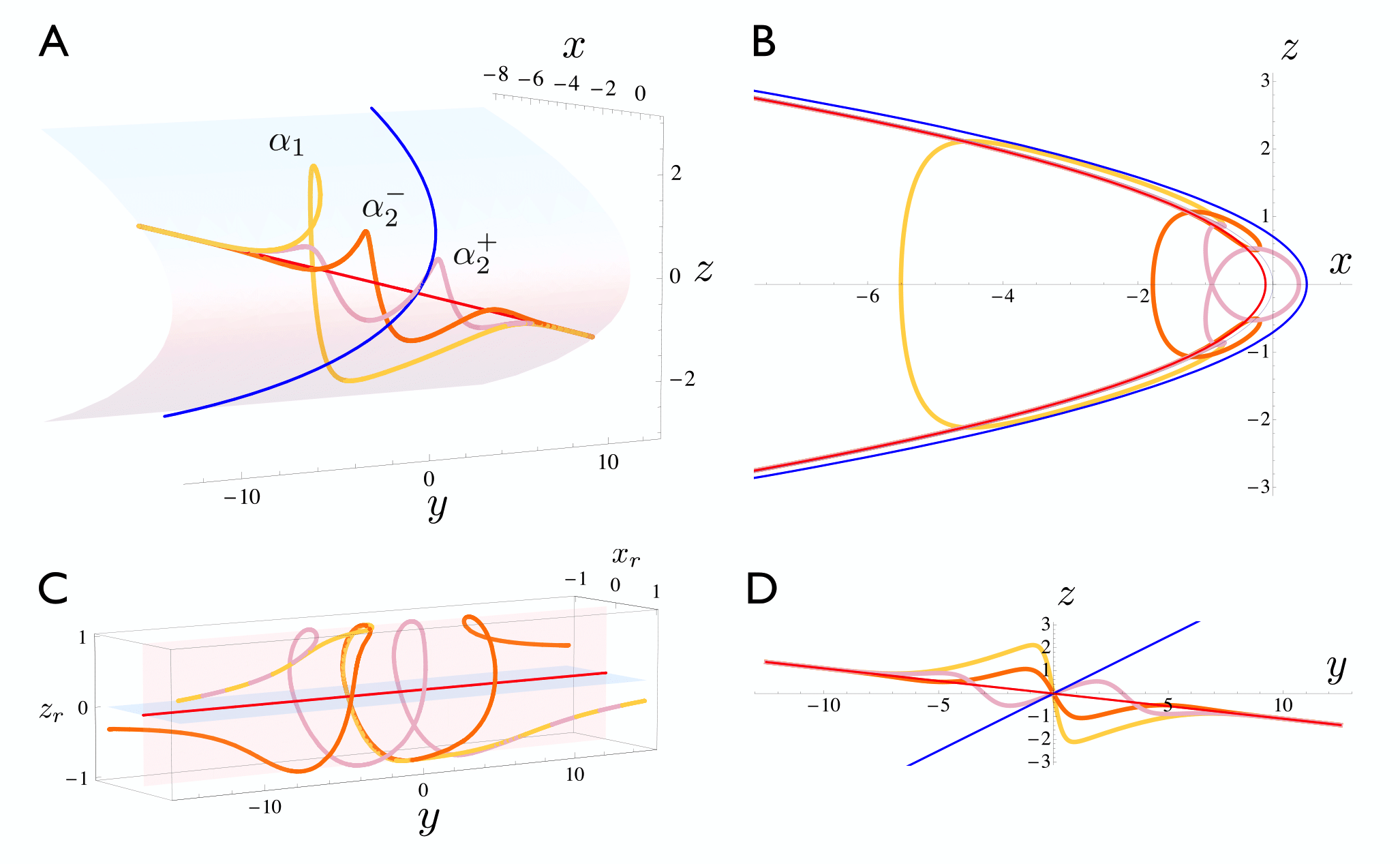
Figure 5: The three \( \alpha \)-faux canards for \( \mu = −0.22 \). Faux canards are shown alongside the true canard \( \gamma_t \) (blue) and the primary faux canard \( \gamma_f \) (red). A: The three \( \alpha \)-faux canards in \( (x,y,z) \)-space. B: Faux canards projected onto \( (x,z) \)-space. C: Faux canards, linearized about the primary faux canard, rescaled to unit distance from \( \gamma_f \) and here shown in \( (x_r,y,z_r) \)-space, where the subscript “r” denotes linearized and rescaled variables. D: Faux canards projected onto \( (y,z) \)-space.
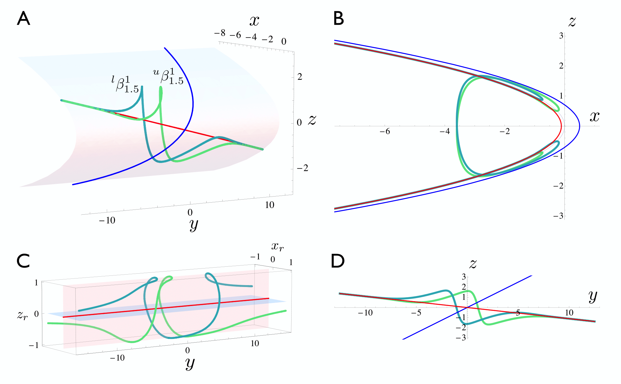
Figure 6: The pair of \( \beta \)-faux canards for \( \mu = −0.22 \). Faux canards are shown alongside the true canard \( \gamma_t \) (blue) and the primary faux canard \( \gamma_f \) (red). A: The two \( \beta \)-faux canards in \( (x,y,z) \)-space. B: Faux canards projected onto \( (x,z) \)-space. C: Faux canards, linearized about the primary faux canard, rescaled to unit distance from \( \gamma_f \) and here shown in \( (x_r,y,z_r) \)-space, where the subscript “r” denotes linearized and rescaled variables. D: Faux canards projected onto \( (y,z) \)-space.
Finally, we note that there exists an additional type of solution which lies at the intersection of a slow manifold and a fast manifold, indicated in blue in Figure 4. These solutions are neither canards nor faux canards, but instead lie completely on one branch of the critical manifold and transition from following the true canard to following the faux canard, or vice versa. We call these solutions \( \chi \)-solutions. Two of the four \( \chi \)-solutions which correspond to the intersections in Figure 4 are shown in Figure 7.
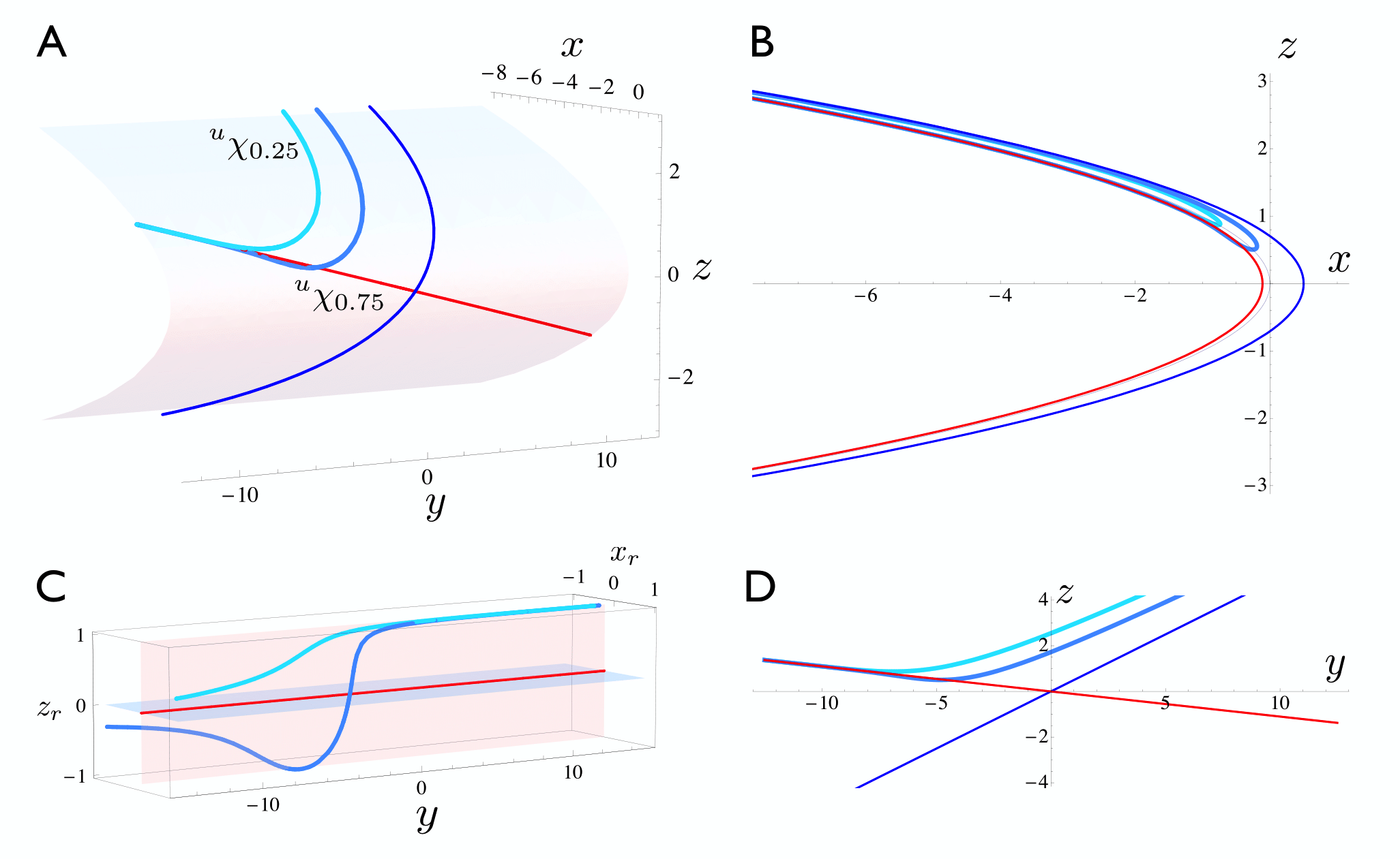
Figure 7: The upper two \( \chi \)-solutions for \( \mu = −0.22 \). \( \chi \)-Solutions are shown alongside the true canard \( \gamma_t \) (blue) and the primary faux canard \( \gamma_f \) (red). A: The upper two \( \chi \)-solutions in (x,y,z)-space. B: \( \chi \)-Solutions projected onto \( (x,z) \)-space. C: \( \chi \)-Solutions, linearized about the primary faux canard, rescaled to unit distance from \( \gamma_f \) and here shown in \( (x_r,y,z_r) \)-space, where the subscript “r” denotes linearized and rescaled variables. D: \( \chi \)-Solutions projected onto (y,z)-space.
The bifurcations of these solutions under variation of \( \mu \) are detailed in [1].
References
[1] J. Mitry, M. Wechselberger, Folded saddles & faux canards, SIAM Journal on Applied Dynamical Systems 16 (2017), 546-596. [doi.org/10.1137/15M1045065]
[2] P. Szmolyan, M. Wechselberger, Canards in R^3, J Differential Equations 177 (2001), 419-453. [doi.org/10.1006/jdeq.2001.4001]
[3] T. Vo, M. Wechselberger, Canards of Folded Saddle-Node Type I, SIAM Journal on Mathematical Analysis 47 (2015), 3235-3283. [doi.org/10.1137/140965818]