In this entry O. E. Omel'chenko, M. Wolfrum, and E. Knobloch summarize an article that they recently published in SIAM Journal on Applied Dynamical Systems [1].

We study destabilization mechanisms of spiral coherence-incoherence patterns known as spiral chimera states that form on a two-dimensional lattice of nonlocally coupled phase oscillators. We consider a model of \( N^2 \) phase oscillators \( \{ \Psi_{jk}(t) \}_{j,k = 1}^N \), evolving according to
(1) \begin{equation}
\frac{d \Psi_{jk}}{dt} = - \sum\limits_{m,n = 1}^N G\left( \frac{2\pi}{N}(j - m), \frac{2\pi}{N}(k - n) \right) \sin\left( \Psi_{jk} - \Psi_{mn} + \alpha \right),
\label{Eq:Oscillators}
\end{equation}
where \( \alpha\in(-\pi/2,\pi/2) \) is the phase lag parameter and \( G \colon \mathbb{R}^2\to\mathbb{R} \) is the coupling function. We take \(G\) to be \(2\pi\)-periodic in both arguments, and employ \(2\pi\)-periodic boundary conditions thereby obtaining patterns on a torus.

We choose, following [2], the coupling function
(2) \begin{equation}
G(x,y) = \cos x + \cos y + \gamma ( \cos 2x + \cos 2y ),\quad \gamma\in\mathbb{R}.
\label{Coupling}
\end{equation}
This coupling function has \( D_4 \) symmetry, given by the reflections \( (x,y)\to (-x,y) \) and \( (x,y)\to (x,-y) \), as well as reflections in the diagonal \( (x,y)\to(y,x) \), and represents a generalization of the case with \( \gamma=1 \) employed in [2].

For suitably chosen initial conditions the system (1)-(2) develops spatio-temporal patterns with self-organized regions of coherent and incoherent motion, called chimera states. We study chimera states consisting of four or \( 16 \) incoherent cores, with each core surrounded by coherent motion in the form of a spiral wave. In each case the incoherent core masks the phase defect at the center of the spiral.

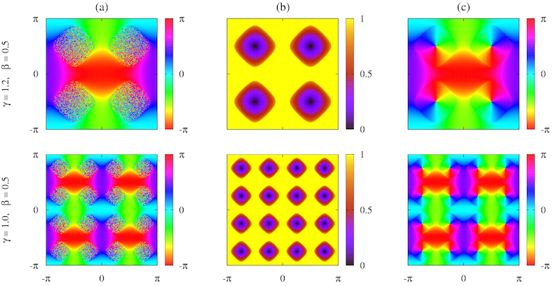
Figure 1: Four-core (upper row) and \( 16 \)-core (lower row) spiral chimeras. (a) Phase snapshots in the system (1)-(2). (b) Modulus and (c) argument of the complex order parameter \( a(x,y) \) of the corresponding rotating wave (5) in the Ott-Antonsen equation (3).

In the large \( N \) limit, the macroscopic dynamics of the system (1)-(2) is described by the Ott-Antonsen equation [3]
(3) \begin{equation}
\frac{d z}{d t} = \frac{1}{2} e^{-i \alpha} \mathcal{G} z - \frac{1}{2} e^{i \alpha} z^2 \mathcal{G} \overline{z}
\label{Eq:OA}
\end{equation}
for the local order parameter \( z(\cdot,t)\in C_\mathrm{per}([-\pi,\pi]^2;\mathbb{C}) \), where
(4) \begin{equation}
(\mathcal{G} z)(x,y,t) := \int_{-\pi}^\pi dx' \int_{-\pi}^\pi G(x-x',y-y') z(x',y',t) dy'
\label{Definition:OperatorG}
\end{equation}
and \( \overline{z} \) denotes the complex conjugate of \( z \). In particular, the spiral chimeras shown in Figure 1(a) correspond to relative equilibria of Eq. (3) with respect to phase shift and are given by the rotating wave ansatz
(5) \begin{equation}
z(x,y,t) = a(x,y) e^{i \Omega t},
\label{Ansatz:Chimera}
\end{equation}
where \( \Omega\in\mathbb{R} \) is the collective frequency and \( a\in C_\mathrm{per}([-\pi,\pi]^2;\mathbb{C}) \) is the stationary spatial profile of the solution. Panels (b) and (c) in Figure 1 show these profiles for the spiral chimeras in Figure 1(a). All profiles lie within the invariant manifold \( |z(x,y,\cdot)|\le 1 \) with \( |a(x,y)| = 1 \) corresponding to the coherent regions of the chimera state and \( |a(x,y)|<1 \) corresponding to the incoherent regions.

The linearization of Eq. (3) around a solution of the form (5) allows us to determine its stability region in the \( (\beta,\gamma) \equiv (\pi/2 -\alpha ,\gamma) \) plane. This is achieved via a matrix characteristic equation, using the finite rank property of the convolution operator \( \mathcal{G} \) defined by (4). 



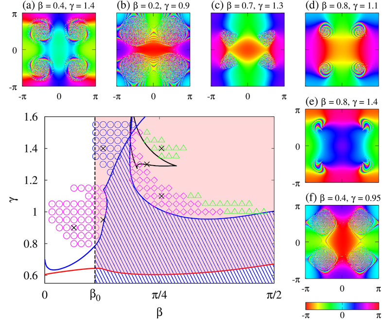
Figure 2. Stability regions of the four-core spiral chimera (hatched) and the \( 16 \)-core spiral chimera (shaded) shown in Figure 1. The former region is bounded by Hopf bifurcation curves (solid blue), and a vertical line of symmetry-breaking bifurcations (\( \beta = \beta_0 \approx 0.34 \), dashed black). The latter region is bounded by a Hopf bifurcation curve (solid red) and a line of symmetry-breaking bifurcations coinciding with that of the four-core spiral chimera. Panels (a)-(f) show the numerically observed patterns at the parameter values given by black crosses. Patterns similar to (a) are observed at locations indicated by blue circles, with patterns similar to (b) indicated by red circles, (d) by red diamonds and (e) by green triangles. For patterns of type (c), the existence region is bounded by the solid black curve. Dynamics of patterns (b), (d) and (f) are shown in the accompanying movies Movie 1, Movie 2, and Movie 3.

Figure 2 summarizes our principal results. It shows the stability regions of the primary spiral patterns in Figure 1(a). The boundaries of these regions consist of two types of curves: Hopf bifurcation curves (solid blue/red curves) and a line of symmetry-breaking bifurcations (black dashed line). All curves have been determined by numerically solving the characteristic equation resulting from the linear stability problem arising from the Ott-Antonsen equation (3).

The side panels in Figure 2 show several other chimera states found by numerical simulation of the system (1)-(2) at locations, indicated with the black crosses, lying outside the hatched stability region of the primary four-core spiral chimera. Each colored symbol refers to one type of pattern and indicates all the parameter values where patterns of this type have been observed. Except for state (c), these patterns can be found numerically by starting with a stable primary spiral chimera and changing parameters quasistatically so as to destabilize this state. On the macroscopic level of the local order parameter, described by the Ott-Antonsen equation (3), these new states turn out to be quasiperiodic and we study them mostly numerically.

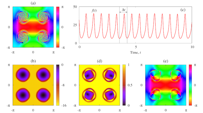
Figure 3. Quasiperiodic spiral chimera. (a) Snapshot of the chimera in the system (1)-(2) for \( N = 256 \), \( \gamma = 1.4 \) and \( \beta = 0.45 \). (b) Mean phase velocities. (c) Indicator function \( f(t) \) for \( (m,n) = (61,30) \) (cross in panel (a)) as defined in (7), showing periodic modulation with a new period \( \Delta t \), where \( \Delta t \) is the time interval between consecutive minima. (d) Modulus and (e) argument of the local order parameter \( Z_{jk} \) evaluated from expression (8).

In Figure 3(a) we show a quasiperiodic spiral chimera resulting from a supercritical Hopf bifurcation of the primary spiral chimera. The state is characterized by a secondary region of coherence located inside the incoherent core of the primary spiral chimera. Primary and secondary coherent regions correspond to frequency-locking plateaus in the profile of the mean phase velocity (panel (b)).

Figure 3 also reveals the second frequency of this quasiperiodic spiral chimera state, corresponding to a relative periodic orbit of the Ott-Antonsen equation (3)
(6)$$
z(x,y,t) = b(x,y,t) e^{i\Omega t},
$$
where \( b(x,y,t) \) is periodic in \( t \) with a period different from \( 2\pi/\Omega \). To extract this new period from numerical simulations of the system (1)-(2) we choose an arbitrary oscillator inside the secondary region of coherence and compare its phase \( \Psi_{mn}(t) \) to the phase of a neighboring oscillator, which we assume to be located inside the secondary region of coherence also. In this way, the quantity
(7)\begin{equation}
f(t) \equiv ( 2\pi / N )^{-1} \sin( \Psi_{mn}(t) - \Psi_{m\: n-1}(t) )
\label{Def:f}
\end{equation}
isolates the new oscillation period that sets in at the Hopf bifurcation (panel (c)).

The successive minima of the indicator function \( f(t) \) define a Poincaré section that can be used to obtain the profile \( b(x,y,\cdot) \) by calculating its average over sufficiently many snapshots. In order to filter out the primary oscillation with the collective frequency \( \Omega \) we subtract from the phase of each oscillator \( \Psi_{jk} \) the phase \( \Psi_\mathrm{coh} \) of an oscillator from the primary coherent region. Denoting by \( S \) the set of instants at which \( f(t) \) attains a local minimum we define the following expression for the local mean field at the grid points:

(8)\begin{equation}
Z_{jk} = \frac{1}{|S|} \sum\limits_{t_l\in S} e^{i ( \Psi_{jk}(t_l) - \Psi_\mathrm{coh}(t_l) )},
\label{LOParam:Experiment}
\end{equation}
where \( |S| \) is the number of elements in \( S \). In Figure 3(d)-(e) we show the modulus and argument of \( Z_{jk} \), representing the modulus and argument of the amplitude \( b(x,y,\cdot) \), respectively.


References

[1] O. E. Omel'chenko, M. Wolfrum and E. Knobloch, Stability of spiral chimera states on a torus, SIAM Journal on Applied Dynamical Systems 17 (2018), 97-127. https://doi.org/10.1137/17M1141151

[2] J. Xie, E. Knobloch and H.-C. Kao, Twisted chimera states and multicore spiral chimera states on a two-dimensional torus, Physical Review E 92 (2015), 042921. https://doi.org/10.1103/PhysRevE.92.042921

[3] E. Ott and T. M. Antonsen, Low dimensional behavior of large systems of globally coupled oscillators, Chaos 18 (2008), 037113. https://doi.org/10.1063/1.2930766