Time series data can arise in many applications, but one area where they naturally appear is dynamical systems.
It can be a signal recorded experimentally, or computed from an underlying mode.
One approach to analyze this data is to map it into a network, where structures of the network capture underlying features of the time series data.
There are numerous methods for how to construct these networks, but here we focus on the ordinal partition graph [7, 3].
Generating an ordinal partition graph from a time series
To generate the ordinal partition graph from a time series \([x_1, \ldots, x_n]\), one must first generate a collection of points \(\mathbf{X} = \{ \mathbf{x}_i = (x_i, x_{i+\tau}, \ldots, x_{i+(d-1)\tau}) \} \subset \mathbb{R}^d\) where \(d\) is the chosen embedding dimension and \(\tau\) is the delay parameter.
Note that this collection of points is the time delay embedding (sometimes called the Takens' embedding) of the time series.
Then for each point \(\mathbf{x}_i = (x_i,\ldots, x_{i+(d-1)\tau})\in \mathbf{X}\), the permutation \(\pi\) of the set \(\{i,i+\tau, \ldots,i+(d-1)\tau\}\) satisfying \(x_{\pi(i)} \leq x_{\pi(i+\tau)}\leq \cdots \leq x_{\pi(i+(d-1)\tau)}\) is associated to \(\mathbf{x}_i\).
Thus, each vector is translated into its associated permutation \(\pi_j\) to generate a collection of permutations where \(j\in \mathbb{Z}\cap [1,n!]\).
The permutations become the vertices in the graph, and an edge \(\pi\pi'\) is added whenever the permutations associated to the ordered point cloud passes between \(\pi\) and \(\pi'\).
A simple example using \(d=3\) can be seen in Fig. 1.
In this case there are six possible permutations which gives six nodes in the network.
Also shown is the permutation sequence, \(P_i\), which records what permutation appears at time \(i\).
Using a higher dimension one can see additional structural detail in the network, such as the example using \(d=7\) shown in Fig. 2.
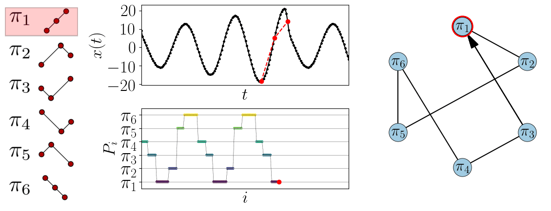
Figure 1: Example of generating the ordinal partition graph from a time series using \(d=3\).
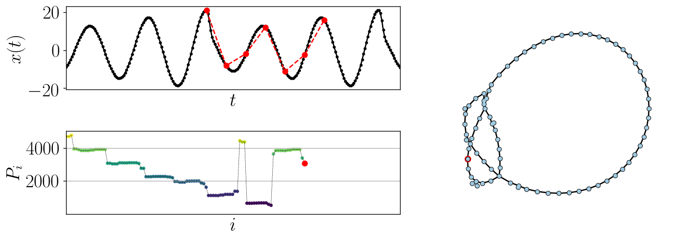
Figure 2: Example of generating the ordinal partition graph from a time series using \(d=7\).
We can also see examples of how the ordinal partition networks behave using time series generated from the Rössler dynamical system:
| |
\( \frac{dx}{dt} = -y-z, \quad \frac{dy}{dt} = x+\alpha y, \quad \frac{dz}{dt} = \beta +z(x-\gamma). \) |
|
Figure 3 shows two time series corresponding to the \(x\)-coordinates of the Rössler system.
These examples are generated using \(\beta=0.2\) and \(\gamma=14\), where \(\alpha=0.1\) in the periodic case, and \(\alpha=0.15\) in the chaotic case.
The initial conditions are set to be \([-0.4, 0.6, 1]\), sampling with a frequency of 15 Hz for 1000 seconds with only the last 170 seconds used to avoid transients.
It is clear in these examples that different types of behavior in time series data appear as structural differences in the corresponding ordinal partition graphs.
There are visual differences in the number of loops and size of the loops in the networks.
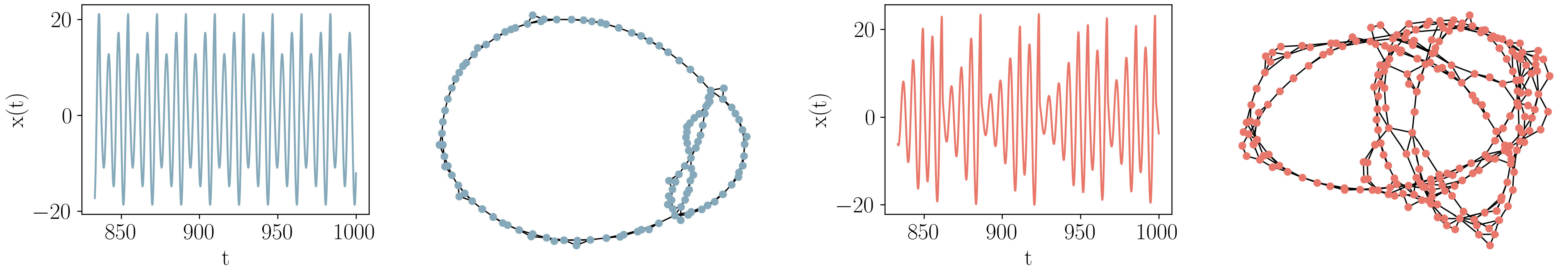
Figure 3: Periodic (left) and chaotic (right) time series generated from the \(x\)-coordinates of the Rössler dynamical system and the corresponding ordinal partition graphs.
Persistent homology of a graph
One tool that can capture these variations comes from the field of Topological Data Analysis (TDA).
Persistent homology summarizes features such as connected components and loops (more precisely, the homology in dimensions 0 and 1 respectively) of a filtered space, often called a filtration.
The output of persistent homology is a persistence diagram, which encodes information about the changing homology.
Here we provide an intuitive explanation of persistent homology, however for a more in depth description we point the reader to [4, 2].
Further a survey of persistent homology of networks can be found in [1].
In order to compute persistent homology, we will generate a sequence of simplicial complexes from a particular network.
A simplicial complex is a space built from vertices and edges (similar to a graph) however additional structure such as triangles between three vertices and their pairwise edges are also allowed.
Given a graph we can construct a simplicial complex at scale \(r\) by adding edges between all pairs of vertices in the graph whose shortest path distance is at most \(r\).
Further, when three pairwise edges are added between three vertices, the triangle between them is also included.
Persistent homology captures how structure changes through the filtration, specifically at what value of \(r\) a circular feature first appears, and at what value of \(r\) the circular feature fills in; these values of \(r\) are called the birth and death time respectively.
The persistence diagram is then a scatter plot of \((r_{birth}, r_{death})\).
An example of a filtration on a network along with the corresponding persistence diagram are shown in Fig. 4.
The persistence diagram encodes the birth and death of several circular features, the most noticeable of which are the two smaller loops, both of which are born at 1 and die at 7, and the larger loop that is born at 1 and dies at 18.
In [6], several experiments are conducted to test how well persistent homology is able to differentiate time series behavior through the topological features captured in the networks.
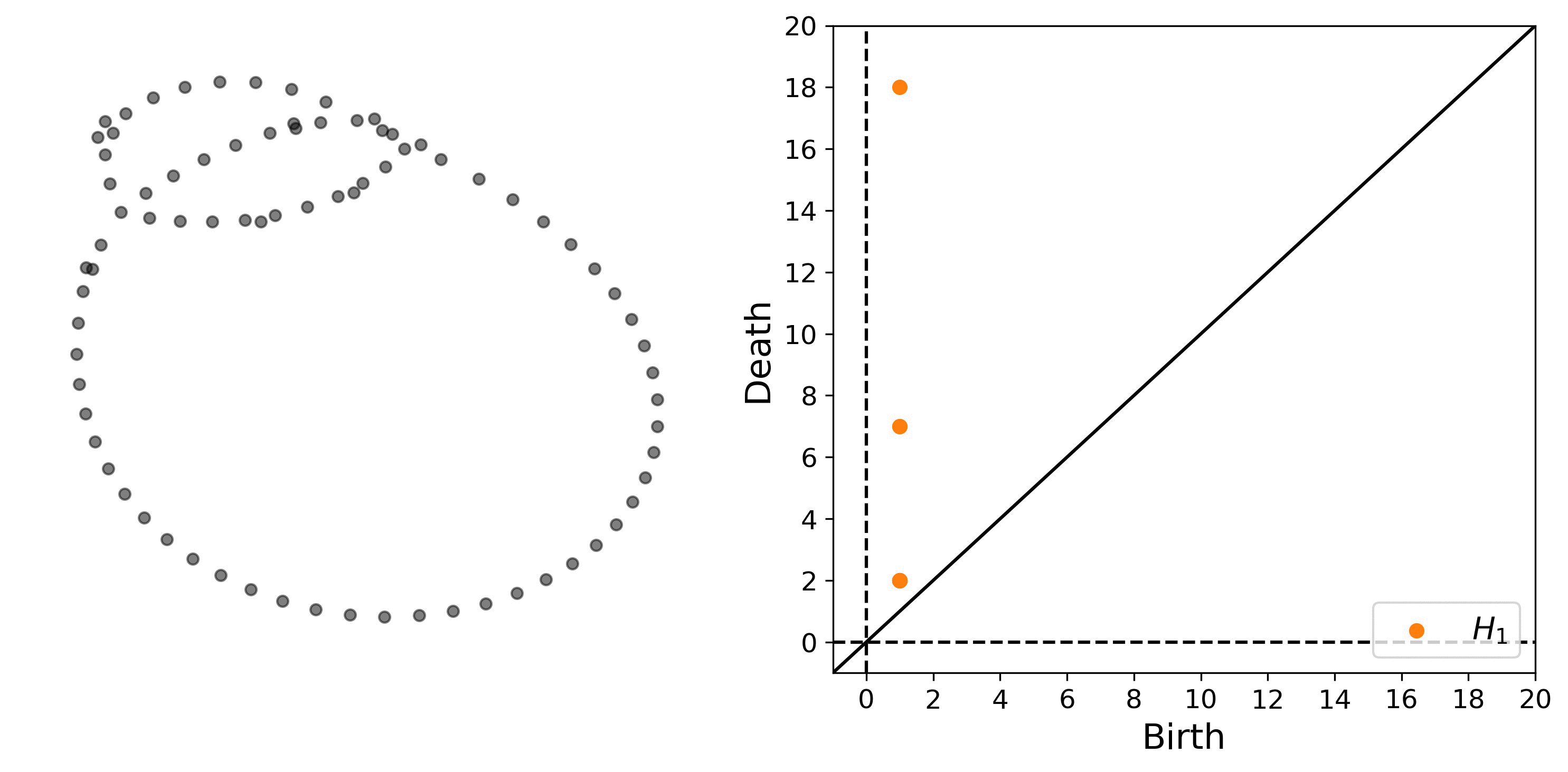
Figure 4: Example of the shortest path distance filtration on a network. Note this network is the ordinal partition graph shown in Fig. 2.
Outlook
There is much more exploration related to work presented here that we will only comment on briefly.
In order to generate the ordinal partition graphs, one must pick two parameters, \(d\) and \(\tau\).
There are many heuristics on how to choose the optimal parameters to reveal the underlying structure in the system.
The one we used in examples shown here is multi-scale permutation entropy which is explained in detail in [5].
Further, ordinal partition graphs can be viewed as weighted, directed networks but incorporating these additional features into a topological analysis is not trivial.
This is the focus of current, ongoing work.
There are also many other types of complex networks that can be generated from time series data [8].
Additional ongoing work is exploring if any of these other methods are well suited to a topological analysis and how they compare to the ordinal partition graph approach described here.
References
[1] Mehmet E. Aktas, Esra Akbas, and Ahmed El Fatmaoui, Persistence homology of networks: methods and applications, Applied Network Science, 4(1), 2019.
[2] Herbert Edelsbrunner and John Harer, Computational Topology: An Introduction, American Mathematical Society, 2010.
[3] Michael McCullough, Michael Small, Thomas Stemler, and Herbert Ho-Ching Iu, Time lagged ordinal partition networks for capturing dynamics of continuous dynamical systems, Chaos: An Interdisciplinary Journal of Nonlinear Science, 25(5), May 2015, p. 053101.
[4] Elizabeth Munch, A user's guide to topological data analysis, Journal of Learning Analytics, 4(2), 2017.
[5] Audun Myers and Firas A. Khasawneh, On the automatic parameter selection for permutation entropy, Chaos: An Interdisciplinary Journal of Nonlinear Science, 30(3), 2020, p. 033130.
[6] Audun Myers, Elizabeth Munch, and Firas A. Khasawneh, Persistent homology of complex networks for dynamic state detection, Physical Review E, 100(2), 2019.
[7] Michael Small, Complex networks from time series: Capturing dynamics, In 2013 IEEE International Symposium on Circuits and Systems (ISCAS2013), IEEE, May 2013.
[8] Minggang Wang and Lixin Tian, From time series to complex networks: The phase space coarse graining, Physica A: Statistical Mechanics and its Applications, 461, 2016, pp. 456–468.
| Author Institutional Affiliation | Michigan State University and Pacific Northwest National Laboratory |
| Author Email | |
| Keywords | time series analysis, topological data analysis, complex networks, chaos, dynamic state, persistent homology, topological signal processing |