1. Introduction and goals
CMlib is a library of cell mapping algorithms and utility functions and classes written in c++. Cell
mapping methods are suitable for the global analysis of dynamical systems, they can be used to
efficiently find state space objects (fixed points, periodic orbits and their corresponding domains of
attractions) in a given discretized state space domain.
The goal of the CMlib library is to provide simple and efficient implementations of basic cell
mapping algorithms allowing users to quickly utilize them to their problems or to integrate them
into other applications independently of the underlying data types or differential equation solvers.
To achieve this, CMlib mostly provides template base classes for various components, from which
application-specific classes can derived.
The target audience of this library (and the included cell mapping methods) ranges from university
students to researchers, as these methods can be used to demonstrate the behaviour of simple
systems or to analyse the state space of complex, non-linear, but usually low-dimensional systems.
The author of the CMlib library have used cell mapping methods extensively during his PhD
studies and currently moving (and rewriting) his private code base to this open-source library.
2. Features
- Current version includes Simple Cell Mapping (SCM) [1] and Clustered SCM [2] methods,
Generalized Cell Mapping (GCM) will be added.
- Entirely written in C++ considering modern language features, with care to code clarity and
documentation.
- Contains cross-platform and efficient implementations of cell mapping algorithms.
- Template approach allows replacing certain components (e.g., underlying data types, methods
for state space discretization, used solvers) easily and independently from each other.
- Open source (with MIT licence), hosted on GitHub.
- Actively maintained and developed.
3. Documentation
The CMlib library is hosted on GitHub at: github.com/Gyebro/cell-mapping.
Doxygen generated code documentation (description of classes, APIs) can be found at the GitHub
page of the repository: gyebro.github.io/cell-mapping.
The latest version of this guide is available in the cell-mapping/docs folder of the repository. The
repository's main page contains information about the currently developed features which can
usually be found on development branches.
4. Installation
4.1. Requirements
The CMlib library can be used as a stand-alone C++ library built from sources contained in the
cpp/cm folder of the repository or as a CMake library. The only requirement is a modern C++
compiler with C++11 support. (GCC 4.8.1 or above, on Windows, MinGW-w64 is recommended.)
For convenience and to aid cross-platform compilation, a CMake project is provided, and it is
recommended to compile the library (and demonstrations) using CMake (available at cmake.org.)
Alternatively, one can use an Integrate Development environment which supports CMake projects,
such as JetBrains CLion (which is available for free to university students and faculty at jetbrains.com/clion).
4.2. Cloning the repository and building the demonstrations
Cloning the CMlib repository can be done with git, or alternatively, by simply downloading the repository as a zip archive.
The top level CMakeLists.txt file can be found in the cell-mapping/cpp folder. For convenience,
scripts for reloading the CMake project (reload-project-* files) and building the demonstrations
(build-demo-* files) are provided.
In order to build the demonstrations on Windows in Release mode, run:
reload-project-release.bat, followed by build-demo-release.bat. To build on Linux, use
the same files with .sh extension.
After building, demonstration executables can be found in the cmake-build-release/demo
folder.
Command line summary:
| git clone https://github.com/Gyebro/cell-mapping.git |
Clone the repository |
| cd cell-mapping/cpp |
Change to project dir |
| reload-project-release.bat |
Reload project in Release |
| build-demo-release.bat |
Build demonstrations |
| cd CMake-build-release/demo |
Change to build dir |
| demo-pendulum |
Run the pendulum demo |
5. Examples
Some simple examples are provided in this section to show the basic concept and usage of the cell
mapping library.
5.1. Simple pendulum
Consider the equation of motion of a simple pendulum with damping \(\delta\) and stiffiness originating
from the gravity (characterised by \(\alpha\)):
| |
\( \ddot{\varphi}(t) + \delta \dot{\varphi} (t) + \alpha \mbox{ sin}(\varphi(t)) = 0 \) |
(1) |
In order to execute Simple Cell Mapping (SCM) on a dynamical system, first a class should be derived from DynamicalSystemBase:
 1  class Pendulum : public cm::DynamicalSystemBase<vec2>  {

2   private:

3    double alpha; // Stiffness

4    double delta; // Damping

5    double dt;    // Target integration time for a "step"

6   public:

7    Pendulum (double alpha, double delta, double timestep) :

8     alpha(alpha), delta(delta) { dt = timestep; }

9    vec2 f(const vec2 &y0, const double& t) const {

10    return vec2({

11     y0[1],

12     -delta*y0[1] -alpha*sin(y0[0])

13    });

14   }

15   vec2 step(const vec2 &state) const override {

16    // Use RK45 to integrate the system scheme

17    cm::RK45<vec2,Pendulum> rk45(this, 1e-8);

18    return rk45.step(state, 0, dt, dt/50.0);

19   }

20 };
The DynamicalSystemBase class requires a step function which can be used to track trajectories
of the system. In order to generate a solution, the RK45 template integrator can be used (see
lines 17-18). To use the solver, the function f(y0,t) needs to be implemented in the Pendulum
class which describes the right-hand side of the system written as a set of first order differential
equations (see lines 11-12). Note: vec2 is a simple 2-element vector type provided by the library.
In order to execute SCM on the Pendulum system, the center, width and cell counts of the state
space along state-space dimensions should be defined. In CMlib, the state space region of interest
is defined by its center point and its width according to Figure 1.
 1  int main () {

2   Pendulum pendulum (1.0, 0.2, 0.1);

3   // Cell state space properties

4   vec2 center = {0.0, 0.0};

5   vec2 width = {16.0*M_PI, 10.0};

6   vector<uint32_t> cells = {1400, 800};

7   // SCM object and solution

8   SCM32<vec2>  scm(center, width, cells, &pendulum);

9   scm.solve(20); // Max. number of steps to leave state-space cells

10  scm.generateImage("pendulum.jpg");

11  return 0;

12 }
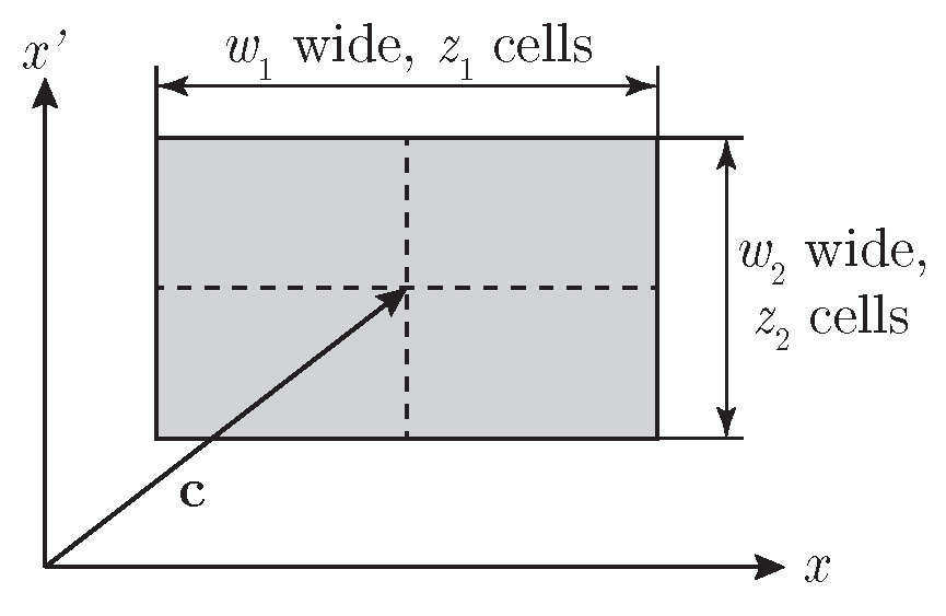
Figure 1. The definition of state space region in \((x, x')\) based on its center c and width w with cell count vector z.
The SCM32<StateVectorType> class' template parameter in this case is vec2 as the Pendulum
used that type for the state vector. Note: SCM32 is a type definition for SCM<SCMCell<uint32_t>,
uint32_t, StateVectorType> meaning, that the addressing of cells are done with 32-bit unsigned
integers. If your state space contains more than \(2^{32} - 1 = 4\) GCells, use SCM64 instead.
After running this example program, the following output is generated:
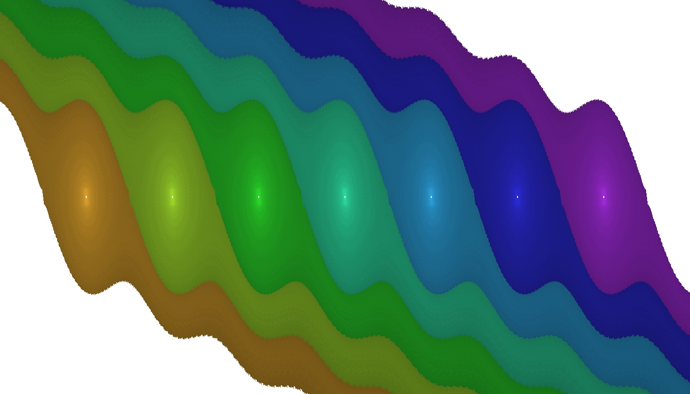
Figure 2. pendulum.jpg: the \((\varphi, \dot{\varphi})\) state space of the simple pendulum. Coloured regions indicate domains of attraction of stable equilibria -- fixed points.
Related files: demo-pendulum.cpp, pendulum.h in the demo folder.
Exercise: Modify the damping parameter of the example and see how the state-space changes.
5.2. Micro-chaos map
Consider a PD-controlled 1 DoF inverted pendulum, where the quantized control force is calculated
at sampling intervals \(\tau\) (zero-order hold). According to the solution of the linearised, dimensionless
equation of motion, the following so-called micro-chaos map can be derived between the states at
subsequent sampling instants:
| |
\( \mathbf{y}_{i+1}=\mathbf{U}\,\mathbf{y}_i+\mathbf{b} \,F_i, \) |
(2) |
where \(F_i=\mathrm{Int}(\hat P x_{i}+\hat D x'_{i})\), \(\mathbf{y}=[x_i\quad x'_i]^T\), and:
\(\begin{equation}
\mathbf{U}=\frac{e^{-\hat{\alpha} \delta}}{\Gamma}
\left[
\begin{array}{cc}
\Gamma \cosh \left(\hat{\alpha } \Gamma \right)+\delta \sinh \left(\hat{\alpha } \Gamma \right) & \sinh \left(\hat{\alpha } \Gamma \right)/\hat{\alpha } \\
\hat{\alpha } \sinh \left(\hat{\alpha } \Gamma \right) & \Gamma \cosh \left(\hat{\alpha } \Gamma \right)-\delta \sinh \left(\hat{\alpha } \Gamma \right) \\
\end{array}
\right], \nonumber
\end{equation}\)
\(\begin{equation}
\mathbf{b}=\frac{1}{{\hat\alpha}^2 \Gamma}\left[\begin{array}{cc}
\Gamma -e^{-\hat{\alpha } \delta } \left(\Gamma \cosh \left(\hat{\alpha } \Gamma \right)+\delta \sinh \left(\hat{\alpha } \Gamma \right)\right) \\
-\hat{\alpha} e^{- \hat{\alpha } \delta }\sinh \left(\hat{\alpha } \Gamma \right)
\end{array}\right] \nonumber
\end{equation}\)
where \(\Gamma=\sqrt{1+\delta^2}\), and \(\hat{\alpha}\) is the dimensionless stiffness, \(\delta\) is the relative damping and \(\hat{P}, \hat{D}\) are the dimensionless control gains. \(\mathrm{Int}()\) denotes taking the integer part of the calculated control effort, and thus introduces switching lines for every integer value.
This system is implemented in the microchaos.h/cpp files in the demo folder of the repository. The system class needs to implement the step function of the DynamicalSystemBase class.
 1 vec2 MicroChaosMapStatic::step(const vec2& y0) const {

2  double F = SymmetricFloor(k*y0); // Rounding at output, k = {P,D}

3  vec2 y1 = U*y0 + b*F;            // The micro-chaos map

4  return y1;

5 }
To apply SCM on this problem, consider the following code snippet:
 1  int main() {

2   double P = 0.007;        // Parameters and system

3   double D = 0.02;

4   double alpha = 0.078;

5   double delta = 0;

6   MicroChaosMapStatic system(P, D, alpha, delta);

7   vec2 center = {0, 0};    // State-space properties

8   vec2 width  = {2400, 50};

9   vector<uint32_t> cells = {1000, 400};

10  SCM32<vec2> scm(center, width, cells, &system); // SCM

11  scm.solve(20);

12  scm.generateImage("scm-microchaos.jpg");

13  return 0;

14 }
After successful execution, the following output image is generated:
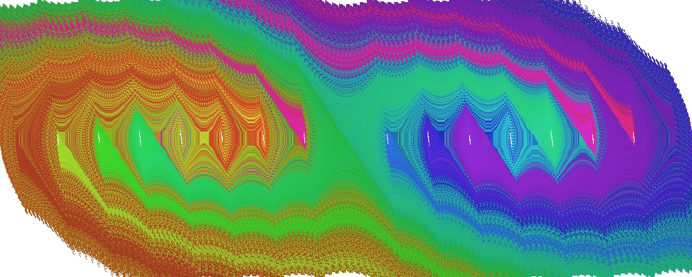
Figure 3. SCM results for the micro-chaos map. Coloured regions indicate domains of attraction of chaotic attractors (white cell groups along the \(x\) axis).
Related files: demo-microchaos.cpp, microchaos.h/cpp in the demo folder.
Exercise: Increase the cell count in the example and see how the tiny details of the state space reveal themselves.
Note: a 4 gigapixel image (corresponding to 4 billion cells, close to the limit of the 32bit unsigned integer address) of this example is hosted at: mm.bme.hu/~gyebro/scm/.
5.3. Duffing oscillator
Consider the Duffing equation:
| |
\( \ddot x(t) + \delta\,\dot x(t) + \alpha x(t) + \beta x^3(t) = \gamma\,\cos(\omega\,t) \) |
(3) |
The implementation of this dynamical system can be found in the duffing.h file. In this example SCM is applied to generate a Poincaré-section of this system by choosing integration time to \(T = 2\,\pi / \omega\).
Consider the following code snippet:
 1  int main() {

2   double alpha = -1.0;      // System and its parameters

3   double beta  = 1.0;

4   double gamma = 0.28;

5   double delta = 0.3;

6   double omega = 1.2;

7   double T = 2*M_PI/omega;

8   DuffingOscillator duffing(alpha, beta, gamma, delta, omega, T);

9

10  vec2 center = {0.0, 0.0}; // Cell state space properties

11  vec2 width  = {4.0, 3.0};

12  vector<uint32_t> cells = {1000, 1000};

13

14  SCM32<vec2> scm(center, width, cells, &duffing);

15  // Declare an alternate coloring method

16  SCMBlackAndWhiteColoring<uint32_t> coloringMethod;

17

18  // Execute SCM with different gamma values

19  vector<double> gammas = {0.28, 0.29, 0.37, 0.5};

20  for (double g : gammas) {

21   duffing.setGamma(g);

22   scm.solve(20);

23   string imageName = "scm-duffing-gamma="+to_string(g)+".jpg";

24   scm.generateImage(imageName, &coloringMethod);

25  }

26  return 0;
Upon successful execution, multiple output images show some characteristic Poincaré-sections of the Duffing equation.
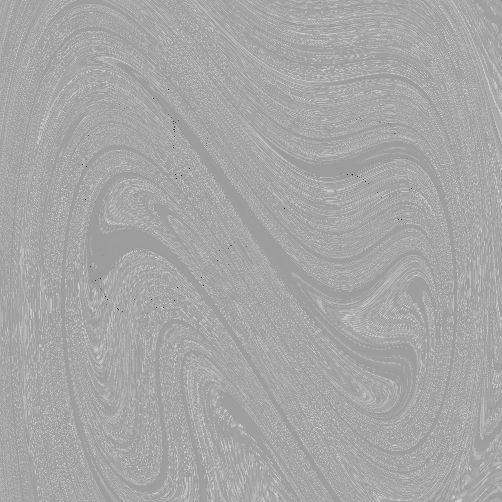
Figure 4. SCM results for the Duffing oscillator's Poincaré-section at \(\gamma = 0.5\).
Related files: demo-duffing.cpp, duffing.h in the demo folder.
Exercise: Run the demo and examine the other outputs. Play with the state space resolution and other system parameters.
References
[1] C. S. Hsu, Cell-to-Cell Mapping: A Method of Global Analysis for Nonlinear Systems, Springer, Singapore, Applied Math. Sciences, 64, 1987. DOI: 10.1007/978-1-4757-3892-6.
[2] G. Gyebrószki and G. Csernák, Clustered Simple Cell Mapping: An extension to the Simple Cell Mapping method, Communications in Nonlinear Science and Numerical Simulation 42, pp. 607–622, 2017. DOI: 10.1016/j.cnsns.2016.06.020.
| Model | |
| Software Type | |
| Language | |
| Platform | |
| Contact Person | |
| References to Papers | [1] C. S. Hsu, Cell-to-Cell Mapping: A Method of Global Analysis for Nonlinear Systems, Springer, Singapore, Applied Math. Sciences, 64, 1987, https://doi.org/10.1007/978-1-4757-3892-6.
[2] G. Gyebrószki and G. Csernák, Clustered Simple Cell Mapping: An extension to the Simple Cell Mapping method, Communications in Nonlinear Science and Numerical Simulation 42, pp. 607–622, 2017, https://doi.org/10.1016/j.cnsns.2016.06.020. |