Eddie Nijholt, Department of Mathematics, University of Illinois, USA ([email protected]).
Bob Rink, Department of Mathematics, Vrije Universiteit Amsterdam, The Netherlands ([email protected]).
Sören Schwenker, Department of Mathematics, University of Hamburg, Germany ([email protected]).

Symmetry can have a major impact on a dynamical system. For instance, a one-dimensional differential equation \(\dot x = F(x)\) with the symmetry \(F(-x)=-F(x)\) will automatically satisfy \(F(0)=0\), and will hence possess a symmetric steady state. This illustrates the principle that symmetric dynamical systems will often have invariant manifolds, such as the fixed point spaces of their symmetry group. More intriguing is the fact that symmetry has a major impact on local bifurcations. The best known example of a symmetry breaking bifurcation is the pitchfork bifurcation

\( \dot x = \lambda x \pm x^3\, . \)

This bifurcation determines how non-symmetric steady states emerge from a symmetric one when an ODE with the symmetry \(F(-x; \lambda)=-F(x;\lambda )\) depends on a varying parameter \(\lambda\).

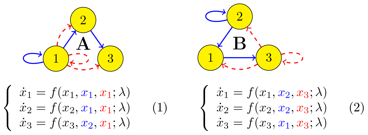
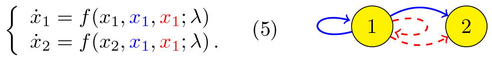
Figure 1. Two networks with identical cells.

It has been noted by many authors that network dynamical systems have very similar characteristics as dynamical systems with symmetry - even if these network systems don't possess any symmetry at all, see [2,3,11]. A good example is synchronisation, seen for instance in the simultaneous firing of neurons. Synchronisation occurs when there is an attracting invariant manifold on which two or more agents in a network exhibit identical behaviour. One doesn't expect to find such an invariant manifold in a dynamical system without symmetry.

Figure 1 depicts two distinct networks and their corresponding ODEs. The function \(f\) depends on a parameter but is otherwise arbitrary. None of the networks appears to have any symmetry. Nevertheless, it is clear from inspecting the ODEs that whenever \(x_1=x_2\), we also have \(\dot x_1 = \dot x_2\). In other words, the synchrony subspace \(\{x_1 = x_2\}\) is an invariant manifold for the dynamics. The same is true for \(\{x_1 = x_2 = x_3\}\). It turns out that bifurcations of synchronous steady states and periodic solutions are highly unconventional as well. Table 1 displays the characteristics of typical one-parameter synchrony breaking steady state bifurcations in these networks.

Network A

Asymptotics	Synchrony
\(x_{1}=x_{2}=x_{3}=0\)	Full
\(x_{1}=x_{2}=0, x_{3} \sim \lambda\)	Partial
\(x_{1}=0, x_{2}\sim \lambda, x_{3} \sim \pm \sqrt{\lambda}\)	None

Network B

Asymptotics	Synchrony
\(x_{1}=x_{2}=x_{3}=0\)	Full
\(x_{1}=x_{2}\sim \lambda, x_{3} \sim \lambda, x_{{1,2}}-x_{3} \sim \lambda\)	Partial
\(x_{1}\sim \lambda, x_{2} \sim \lambda, x_{3} \sim \lambda\) \(x_{1}-x_{2}\sim \lambda^2, x_{{1,2}}-x_{3} \sim \lambda\)	None but almost partial

Table 1. Asymptotics of the three steady state branches that coalesce in a typical one-parameter synchrony breaking bifurcation at the fully synchronous state \((x;\lambda)=(0;0)\).

We found that some of these phenomena in networks, including synchronisation and anomalous synchrony breaking bifurcations, are caused by an unusual type of generalised symmetry.

Definition: An ODE with generalised symmetry consists of a finite collection of ODEs

\( \dot x = F_v(x)\ \mbox{with}\ x\in \mathbb{R}^{n_v}\, , \)

for \(v\) in some set \(V\), and a finite collection of linear maps

\( R_a: \mathbb{R}^{n_{s(a)}} \to \mathbb{R}^{n_{t(a)}}\, , \)

for \(a\) in some set \(A\), and with \(s(a), t(a) \in V\). Each map \(R_a\) moreover sends orbits of \(F_{s(a)}\) to orbits of \(F_{t(a)}\), i.e.,

\( R_a\circ F_{s(a)} = F_{t(a)} \circ R_a\, \mbox{for all}\ a\in A\, . \)

The notation suggests that the \(v\in V\) are vertices and the \(a\in A\) are arrows of a directed graph \((V,A)\), where \(s(a), t(a)\) denote the source and target vertex of the arrow \(a\). Such a symmetry structure encoded by a directed graph is also called a quiver representation.

A very simple non-classical example of generalised symmetry (where the symmetry does not form a group) is actually well known. Suppose we only have one vertex \(v\in V\) and a single arrow \(a\in A\), and consider the map

\( R_a: x\mapsto 0\ \mbox{from}\ \mathbb{R}\ \mbox{to}\ \mathbb{R}\, . \)

An ODE \(\dot x = F_v(x)\) satisfies \(F_v\circ R_a = R_a \circ F_v\) if and only if \(F_v(0)=0\). So having this symmetry is equivalent to having a steady state at the origin. The transcritical bifurcation

\( \dot x = \lambda x \pm x^2 \)

is the typical one-parameter bifurcation in this setting. What this shows is that the transcritical bifurcation is actually a generalised symmetric bifurcation!

Generalised symmetry in networks

Generalised symmetry provides an alternative explanation for the invariant synchrony spaces \(\{x_1=x_2\}\) and \(\{x_1=x_2=x_3\}\) of networks (1) and (2). Consider the ODE

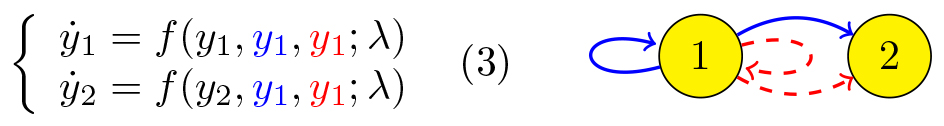
and note that when \((y_1(t), y_2(t))\) is a solution of (3), then

\( (x_1(t), x_2(t), x_3(t)):= (y_1(t), y_1(t), y_2(t)) \)

is a solution of (1). In other words, the map

\( R_{a_1}: (y_1, y_2) \mapsto (x_1, x_2, x_3) := (y_1, y_1, y_2) \)

sends solutions to solutions and is therefore a generalised symmetry. Its image is precisely the synchrony space \(\{x_1=x_2\}\). Similarly, the map

\( R_{a_2}: z_1\mapsto (y_1, y_2):=(z_1,z_1) \)

is a generalised symmetry that turns solutions of

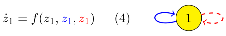
into fully synchronous solutions of (3).

Equations (3) and (4) define what are called quotients of network A, cf. [1,3,11,12]. Figure 2 depicts all the quotients of networks A and B. Quotient networks were introduced by Golubitsky, Stewart et al. [12]. In [1] it was noted for the first time that quotient networks are the same thing as injective generalised symmetries.

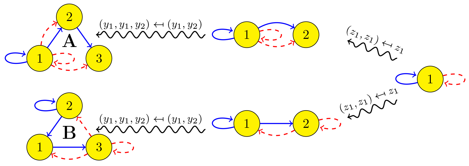
Figure 2. Quotients of networks A and B.

Another class of generalised symmetries arise from subnetworks. A subnetwork is a subset of the cells that does not receive inputs from cells outside of it. Network A is a so-called feedforward network, a type of network known to have relatively many subnetworks. Cells 1 and 2, for example, are not influenced by cell 3. This implies that the surjective map

\( R_{a_3}: (x_1, x_2, x_3)\mapsto (x_1, x_2) \)

sends solutions of (1) to solutions of

Network A has two nontrivial subnetworks in total, giving rise to two generalised symmetries, see Figure 3. Network B has no subnetworks.

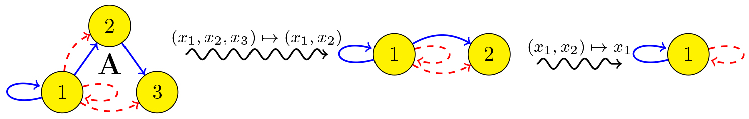
Figure 3. Subnetworks of network A.

Why is generalised symmetry of interest?

Our goal is to understand how the network structure of an ODE impacts its dynamical behaviour. In general this is very unclear, most notably because the exact network structure of an ODE is usually destroyed when one makes coordinate transformations. Generalised symmetry on the other hand is an intrinsic geometric property, and is therefore much easier to incorporate in for instance bifurcation analysis.

We have for example shown that generalised symmetry can be preserved in center manifold reduction [6] and Lyapunov-Schmidt reduction [8]. Generalised symmetry thus puts restrictions on the equations that determine the solution branches that emerge in a bifurcation, in exactly the same way that symmetry determines the pitchfork and transcritical bifurcation. The following unpublished result shows that generalised symmetry is compatible with normal form reduction.

Theorem 0.1. [Generalised symmetry normal form theorem]

Consider a collection of ODEs \(\dot x = F_v(x)\) (for \(v\in V\)) with Taylor expansions

\( F_v(x) = F^1_v(x) + F^2_v(x) + \ldots\, . \)

Here \(F^1_v\) is linear, \(F_v^2\) quadratic, etc. Assume that \(F_{t(a)}\circ R_a = R_a \circ F_{s(a)}\) for all \(a\in A\). Then for each \(1\leq m <\infty\) there exist local coordinate changes \(x\mapsto y = \Phi_v(x)\) transforming these ODEs into the form \(\dot y = \overline F_v(y)\), where

\( \overline F_v(y) = \overline F^1_v(y) + \overline F^2_v(y) + \ldots \ , \)

and such that

1. generalised symmetry is preserved: \(R_a \circ \overline{F}_{s(a)} = \overline{F}_{t(a)}\circ R_a\) for all \(a\in A\);
2. each \(\overline F^k_v\ ( 1\leq k \leq m)\) commutes with the semi-simple part of \(\overline F^1_v\).

This result implies that quotients, subnetworks and all sorts of other generalised symmetry can be preserved in the normal form. We have used a weaker version of this theorem [9] to classify Hopf bifurcations in a class of feedforward networks [7].

Quotient networks and subnetworks are among the simplest types of generalised symmetries to be found in networks. Much less intuitive are the so-called hidden symmetries discovered in [4,8] and subsequently analysed in [5,6,9,10]. An example is the map

\( R_{a_4}: (x_1, x_2, x_3)\mapsto (x_1, x_1, x_2) \)

that sends solutions of (1) to solutions of (1). We proved that this unusual non-invertible transformation is responsible for the bifurcation of network A shown in Table 1. The situation is even more intricate for network B. It turns out that this network is the quotient of a network C that admits four non-invertible symmetries, see Figure 4. This hidden network C is responsible for the bifurcations in network B presented in Table 1.

Our aim is to exploit generalised symmetries to classify many more such remarkable synchrony breaking bifurcations in network systems.

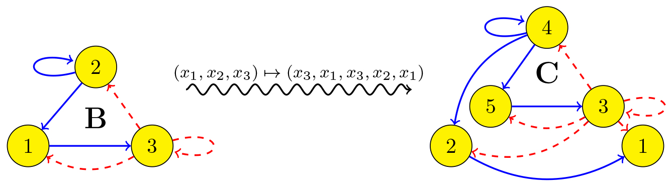
Figure 4. The hidden network C determines the bifurcations in network B.

Acknowledgements

Bob Rink is happy to acknowledge the hospitality and financial support of the Sydney Mathematical Research Institute. This research is partly financed by the Dutch Research Council (NWO) through Eddie Nijholt's research program "Designing Network Dynamical Systems through Algebra".

References

[1]   L. Deville and E. Lerman, Modular dynamical systems on networks, J. Eur. Math. Soc., 17 (2015), pp. 2977–3013.

[2]   M. Field, Combinatorial dynamics, Dyn. Syst., 19 (2004), pp. 217–243, https://doi.org/10.1080/14689360410001729379.

[3]   M. Golubitsky, M. Nicol, and I. Stewart, Some curious phenomena in coupled cell networks, J. Nonlinear Sci., 14 (2004), pp. 207–236, https://doi.org/10.1007/s00332-003-0593-6.

[4]   E. Nijholt, B. Rink, and J. Sanders, Graph fibrations and symmetries of network dynamics, J. Differ. Equations, 261 (2016), pp. 4861–4896.

[5]   E. Nijholt, B. Rink, and J. Sanders, Projection blocks in homogeneous coupled cell networks, Dyn. Syst., 32 (2017), pp. 164–186, https://doi.org/10.1080/14689367.2016.1274018.

[6]   E. Nijholt, B. Rink, and J. Sanders, Center manifolds of coupled cell networks, SIAM Review, 61 (2019), pp. 121–155.

[7]   B. Rink and J. Sanders, Amplified hopf bifurcations in feed-forward networks, SIAM J. Appl. Dyn. Syst., 12 (2013), pp. 1135–1157.

[8]   B. Rink and J. Sanders, Coupled cell networks and their hidden symmetries, SIAM J. Math. Anal., 46 (2014), pp. 1577–1609.

[9]   B. Rink and J. Sanders, Coupled cell networks: semigroups, Lie algebras and normal forms, Trans. Amer. Math. Soc., 367 (2015), pp. 3509–3548.

[10]   S. Schwenker, Generic steady state bifurcations in monoid equivariant dynamics with applications in homogeneous coupled cell systems, SIAM J. Math. Anal., 50 (2018), pp. 2466–2485.

[11]   I. Stewart, Networking opportunity, Nature, 427 (2004), pp. 601–604.

[12]   I. Stewart, M. Golubitsky, and M. Pivato, Symmetry groupoids and patterns of synchrony in coupled cell networks, SIAM J. Appl. Dyn. Syst., 2 (2003), pp. 609–646, https://doi.org/10.1137/S1111111103419896.