1. Introduction
PyDMD - Python Dynamic Mode Decomposition [4] is a
Python package that uses Dynamic Mode Decomposition for a data-driven
model simplification based on spatiotemporal coherent structures.
Dynamic Mode Decomposition (DMD) is a model reduction algorithm
developed by Schmid [15]. Since then it has emerged
as a powerful tool for analyzing the dynamics of nonlinear
systems. DMD relies only on the high-fidelity measurements, like
experimental data and numerical simulations, so it is an equation-free
algorithm. Its popularity is also due to the fact that it does not
make any assumptions about the underlying system. See
Kutz [9] for a comprehensive overview of the
algorithm and its connections to the Koopman-operator analysis,
initiated in Koopman [8], along with
examples in computational fluid dynamics.
In the last years many variants arose, such as multiresolution
DMD [10], compressed
DMD [5], DMD with
control [13], forward backward
DMD, sparsity promoting DMD to choose dynamically
important DMD modes [7], and higher
order DMD [11] among others, in order to deal with
noisy data, big datasets, or spurious data for example.
In the PyDMD package we implemented in Python the
majority of the variants mentioned above with a user friendly interface. We also
provide many tutorials that show all the characteristics of the
software, ranging from the basic use case to the most sophisticated one
allowed by the package.
The research in the field is growing both in computational fluid
dynamic and in structural mechanics, due to the equation-free nature
of the model. We cite among others, applications in the framework of shape
optimization in naval
engineering [2, 16, 3]. For
numerical non-intrusive pipelines for applied sciences and industrial
application we cite [14, 17].
2. Main features
The main important features of the PyDMD package are the following:
- Thoroughly documented, with an easily accessible online
documentation.
- Modular package easily integrable into existing computational
pipelines.
- Fast learning rate due to the simplicity of the code design
inspired by scikit-learn.
- No external dependencies. It uses only standard and well spread
Python packages.
- Written following the Python programming best practices.
- Open source software, distributed via GitHub. This ensures an easy
contributing procedure and issue tracking.
- A permissive free software license (MIT License), with an
excellent license compatibility.
- A vast amount of tutorials.
3. Installation
PyDMD requires numpy, scipy, matplotlib, future, sphinx (for local documentation) and nose
(for local test). The code is compatible with Python 2.7 and Python
3.6. It can be installed using pip or directly from the source code.
Mac and Linux users can install pre-built binary packages using pip. To install the package just type:
pip install pydmd
To uninstall the package:
pip uninstall pydmd
It is also possible to install the package locally, after cloning it, for example during
the developing stage of new features, with
 git clone https://github.com/mathLab/PyDMD


python setup.py install
or, in alternative, to install the latest version on the master branch
on GitHub use the following command
pip install git+https://github.com/mathLab/PyDMD.git
4. Documentation
PyDMD uses sphinx for code documentation. You can view the
documentation online here: https://mathlab.github.io/PyDMD/. To
build the html version of the docs locally simply type the following
from within the pydmd folder:
 cd docs


make html
The generated html can be found in docs/build/html. Open up the index.html file you find there to browse the documentation.
5. Testing
We are using Travis CI for continuous integration testing for Mac and
Linux platforms and for Python 2.7 and 3.6. You can check out the
current status here: https://travis-ci.org/mathLab/PyDMD. To run tests locally (nose is required):
python test.py
6. Tutorials
We are going to present the main features of the software following some of the tutorials available online. First we introduce mathematically the algorithm, then in the following subsections we start with the basic usage of the classical DMD, then we introduce more advanced options we can pass to the base class, and finally we show how to use the DMD variants we implemented. All the tutorials can be found online in the GitHub repository at https://github.com/mathLab/PyDMD/tree/master/tutorials.
6.1 Mathematical formulation
The dynamic mode decomposition is a powerful method that allows the approximation of complex
nonlinear systems as the combination of low-rank structures evolve linearly
in time. These structures, called modes, and their time
evolution, called dynamics, come from the decomposition, based on the
(SVD), of the output data of the studied system. Relying only on the
high-fidelity measurements (experimental data, numerical simulations), the
DMD has the big benefit of being an equation-free algorithm, and it does
not make assumptions about the underlying system.
Due to the complex systems simplification through the dynamics modes, this
method gives us the possibility to
- better understand the model thanks to the analysis of the low-rank
spatiotemporal features extracted, as we are going to show in Section 6.2;
- accurately reconstruct the temporal evolution of the system and a
short-time future estimation.
The basic idea behind DMD is to approximate the evolution of the complex
system with a linear operator \(\mathbf{A}\) such that \(x_{k+1} =
\mathbf{A}x_k\), where \(x_k \in \mathbb{R}^n\) is the vector
representing the state of the system at time \(k\). We underline that
the state vectors are equispaced in time. To obtain the minimum
approximation error across all these snapshots, it is possible to
arrange them in two matrices as following:
| |
\begin{equation}
\mathbf{X} =
\begin{bmatrix}
x_1^1 & x_2^1 & \cdots & x_{m-1}^1 \\
x_1^2 & x_2^2 & \cdots & x_{m-1}^2 \\
\vdots & \vdots & \ddots & \vdots \\
x_1^n & x_2^n & \cdots & x_{m-1}^n
\end{bmatrix},\quad\quad
\mathbf{Y} =
\begin{bmatrix}
x_2^1 & x_3^1 & \cdots & x_m^1 \\
x_2^2 & x_3^2 & \cdots & x_m^2 \\
\vdots & \vdots & \ddots & \vdots \\
x_2^n & x_3^n & \cdots & x_m^n
\end{bmatrix}.
\end{equation} |
(1) |
In this way, each column of \(\mathbf{Y}\) contains the state vector at
the next timestep of the one in the corresponding \(\mathbf{X}\)
column.
We underline that the snapshots are sampling the evolution of a nonlinear
system and we are looking for a linear operator. Thus, we want to find
\(\mathbf{A}\) such that \(\mathbf{Y} \approx \mathbf{A} \mathbf{X}\).
The best-fit \(\mathbf{A}\) matrix is given by \(\mathbf{A} = \mathbf{Y}
\mathbf{X}^\dagger\), where the symbol \(^\dagger\) denotes the
Moore-Penrose pseudo-inverse.
Since the snapshots \(x_i\) represent the state of the system, we assume
they are high dimensional: hence the matrix \(\mathbf{A}\) has \(n^2\)
elements (supposing the dimension \(n\) of a snapshot is larger than the
number of snapshots \(m\)) and it is difficult to decompose or to
handle. The DMD algorithm projects the data onto a low-rank subspace
defined by the proper orthogonal decomposition (POD) modes, then computes the low-dimensional operator
\(\tilde{\mathbf{A}}\); finally this operator is used to reconstruct the leading
nonzero eigenvalues and eigenvectors of the full-dimensional operator
\(\mathbf{A}\) without ever explicitly computing \(\mathbf{A}\).
First, we compute the truncated (SVD) of the matrix \(\mathbf{X}\):
| |
\(\mathbf{X} \approx \mathbf{U}_r \mathbf{\Sigma}_r \mathbf{V}^*_r ,\) |
(2) |
where \(\mathbf{U}_r \in \mathbb{C}^{n\times r}\), \(\mathbf{\Sigma}_r \in
\mathbb{C}^{r\times r}\) and \(\mathbf{V}_r \in \mathbb{C}^{m\times r}\). Here \(r\)
is the rank of the reduced (SVD) approximation and \(^*\) denotes the
conjugate transpose. The columns of \(\mathbf{U}_r\) are orthonormal and they are
the first \(r\) (POD) modes, so we can use the matrix \(\mathbf{U}_r\) to build
the low-dimensional operator \(\mathbf{\tilde{A}}\). Recalling the definition of
\(\mathbf{A}\) and the decomposition of \(\mathbf{X}\) we obtain
| |
\(\mathbf{\tilde{A}} = \mathbf{U}_r^* \mathbf{Y} \mathbf{V}_r \mathbf{\Sigma}_r^{-1}.\) |
(3) |
Avoiding the explicit calculation of the high-dimensional operator
\(\mathbf{A}\), we obtain the matrix \(\mathbf{\tilde{A}} \in \mathbb{C}^{r\times
r}\) that defines the linear evolution of the low-dimensional model as
\(\tilde{x}_{k+1} = \mathbf{\tilde{A}} \tilde{x}_k\),
where \(\tilde{x}_k\) is the low-rank approximated state. It is possible
reconstruct the high-dimensional state \(x_k\) as \(x_k = \mathbf{U}_r\tilde{x}_k\).
Thanks to the eigendecomposition of \(\mathbf{\tilde{A}}\)
| |
\(\mathbf{\tilde{A}} \mathbf{W} = \mathbf{W} \mathbf{\Lambda}\) |
(4) |
we can reconstruct the eigenvectors and eigenvalues of the matrix \(\mathbf{A}\). In particular, the eigenvectors can be computed in two ways:
- the eigenvectors of \(\mathbf{A}\) are reconstructed by projecting
the low-rank approximation \(\mathbf{W}\) on the high-dimensional
space: \(\mathbf{\Phi} = \mathbf{U}_r \mathbf{W}\).
We call the eigenvectors computed in this way the projected (DMD)
modes.
- the so called exact (DMD) modes, the real eigenvectors of
\(\mathbf{A}\), are instead the columns of \(\mathbf{\Phi} = \mathbf{Y}\mathbf{V}_r \mathbf{\Sigma}_r^{-1} \mathbf{W}\).
To demonstrate the relation between the exact (DMD) modes and the
eigenvectors of the matrix \(\mathbf{\tilde{A}}\), we recall the
eigendecomposition of the high-dimensional operator and the definitions
\(\mathbf{A}= \mathbf{Y} \mathbf{V}_r \mathbf{\Sigma}^{-1}_r \mathbf{U}^*_r\) and
\(\mathbf{\tilde{A}} = \mathbf{U}^*_r \mathbf{Y} \mathbf{V}_r
\mathbf{\Sigma}^{-1}_r\):
| |
\begin{equation}
\begin{split}
\mathbf{A} \mathbf{\Phi} &= \mathbf{\Phi} \mathbf{\Lambda}\\
\mathbf{A} \mathbf{Y}\mathbf{V}_r \mathbf{\Sigma}_r^{-1} \mathbf{W} &=
\mathbf{Y} \mathbf{V}_r \mathbf{\Sigma}_r^{-1} \mathbf{W} \mathbf{\Lambda}\\
\mathbf{Y} \mathbf{V}_r \mathbf{\Sigma}_r^{-1} \mathbf{U}^*_r
\mathbf{Y}\mathbf{V}_r \mathbf{\Sigma}_r^{-1} \mathbf{W} &=
\mathbf{Y}\mathbf{V}_r \mathbf{\Sigma}_r^{-1} \mathbf{W} \mathbf{\Lambda}\\
\mathbf{Y} \mathbf{V}_r \mathbf{\Sigma}_r^{-1} \mathbf{\tilde{A}}
\mathbf{W} &= \mathbf{Y}\mathbf{V}_r \mathbf{\Sigma}_r^{-1} \mathbf{W}
\mathbf{\Lambda}\\
\mathbf{\tilde{A}} \mathbf{W} &= \mathbf{W} \mathbf{\Lambda}.
\end{split}
\end{equation} |
(5) |
This also proves that the eigenvalues
obtained from the decomposition of \(\mathbf{\tilde{A}}\) coincide with the
eigenvalues of \(\mathbf{A}\). These eigenvalues \(\mathbf{\Lambda} =
\begin{bmatrix}\lambda_0&\lambda_1&\dotsc&\lambda_r\end{bmatrix}\) with
\(\lambda_i \in \mathbb{C}\) for \(i = 0,1,\dotsc,r\), contain
growth/decay rates and frequencies of the corresponding DMD modes.
We use the eigendecomposition to rewrite the definition of the linear operator:
| |
\begin{equation}
\begin{split}
\mathbf{Y} &\approx \mathbf{A} \mathbf{X}\\
&\approx \mathbf{\Phi} \mathbf{\Lambda} \mathbf{\Phi}^\dagger \mathbf{X}\\
&\approx \mathbf{\Phi} \mathbf{\Lambda} \mathbf{\Phi}^\dagger
\begin{bmatrix}\mathbf{x}_0 & \mathbf{x}_1 & \mathbf{x}_2 & \dotsc &
\mathbf{x}_r\end{bmatrix}\\
&\approx \mathbf{\Phi}\mathbf{\Lambda} \mathbf{\Phi}^\dagger
\begin{bmatrix}\mathbf{x}_0 & \mathbf{A}\mathbf{x}_0 &
\mathbf{A}^2\mathbf{x}_0& \dotsc & \mathbf{A}^{r-1}\mathbf{x}_0\end{bmatrix}\\
&\approx \mathbf{\Phi}\mathbf{\Lambda} \mathbf{\Phi}^\dagger
\begin{bmatrix}
\mathbf{x}_0 &
\mathbf{\Phi}\mathbf{\Lambda}\mathbf{\Phi}^\dagger\mathbf{x}_0 &
\mathbf{\Phi}\mathbf{\Lambda}\mathbf{\Phi}^\dagger
\mathbf{\Phi}\mathbf{\Lambda} \mathbf{\Phi}^\dagger\mathbf{x}_0&
\dotsc &
(\mathbf{\Phi}\mathbf{\Lambda}\mathbf{\Phi}^\dagger)^{r-1}\mathbf{x}_0
\end{bmatrix}\\
&\approx \mathbf{\Phi}\mathbf{\Lambda}
\begin{bmatrix}
\mathbf{b} &
\mathbf{\Lambda}\mathbf{b} &
\mathbf{\Lambda}^2\mathbf{b} &
\dotsc&
\mathbf{\Lambda}^{r-1}\mathbf{b}
\end{bmatrix}\\
&\approx \mathbf{\Phi}
\begin{bmatrix}
\mathbf{\Lambda} &
\mathbf{\Lambda}^2&
\dotsc&
\mathbf{\Lambda}^{r}
\end{bmatrix}
\mathbf{b}
\end{split}
\end{equation} |
(6) |
where \(\mathbf{b}\) refers to the amplitudes of the first snapshot such that
\(\mathbf{b} = \mathbf{\Phi}^\dagger \mathbf{x}_0\). Thus, it is
possible to approximate the state of the system at the generic time
\(t_k = k\Delta t\) by computing \(\mathbf{x}_k = \mathbf{\Phi}
\mathbf{\Lambda}^k \mathbf{b}\).
6.2 How to use the standard algorithm
In the following tutorial, we apply the standard DMD to a very simple system in order to
show the capabilities of the algorithm and the package interface.
We create the input data by summing the following two functions
| |
\begin{equation}
\begin{split}
f_1(x,t) &=\mbox{sech}(x+3)\exp(i2.3t),\\
f_2(x,t) &=2\mbox{sech}(x)\tanh(x)\exp(i2.8t).\\
\end{split}
\end{equation} |
(7) |
and we import the PyDMD environment and in particular the DMD class using the code below.
  import matplotlib.pyplot as plt

import numpy as np


from pydmd import DMD


def f1(x,t):


return 1./np.cosh(x+3)*np.exp(2.3j*t)


def f2(x,t):


return 2./np.cosh(x)*np.tanh(x)*np.exp(2.8j*t)


x = np.linspace(-5, 5, 128)

t = np.linspace(0, 4*np.pi, 256)

xgrid, tgrid = np.meshgrid(x, t)


X1 = f1(xgrid, tgrid)

X2 = f2(xgrid, tgrid)

X = X1 + X2
Now we have the temporal snapshots in the input matrix rows: we can easily
create a new DMD instance and exploit it in order to compute the decomposition
on the data. Since the snapshots must be arranged by columns, in this case we
need to transpose the matrix.
 dmd = DMD(svd_rank=2)

dmd.fit(X.T)
The dmd object contains the principal information about the decomposition:
- the attribute modes is a 2D numpy array where the columns are the
low-rank structures individuated;
- the attribute dynamics is a 2D numpy array where the rows refer to the
time evolution of each mode;
- the attribute eigs refers to the eigenvalues of the low
dimensional operator;
- the attribute reconstructed_data refers to the approximated system
evolution.
We are able to easily visualise the eigenvalues using the method
plot_eigs or plotting the modes and the dynamics thanks to
matplotlib library, as shown in Figure 1.
 for mode in dmd.modes.T:


plt.plot(x, mode.real)


plt.title('Modes')

plt.show()


for dynamic in dmd.dynamics:


plt.plot(t, dynamic.real)


plt.title('Dynamics')

plt.show()
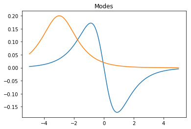
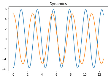
Figure 1. The DMD modes and the corresponding dynamics.
Finally, we can reconstruct the original dataset as the product of modes and
dynamics. In Figure 2 we plot the evolution of each mode to emphasize
their similarity with the input functions and we plot the reconstructed data.
Figure 2. The application of the DMD algorithm on the toy dataset: the
evolving system is simulated summing \(f_1\) and \(f_2\); the two dynamics coincide with these functions and the target dynamical system is faithfully reconstructed.
6.3 More advanced options
We create the dataset with an hyperbolic secant with damped oscillations
as in the following formula:
| |
\(f(x, y, t) = \mbox{sech}(x) \mbox{sech}(y) 2.4 i^{-t} + r\) |
(8) |
where \(r\) is a random noise term sampled from a normal (Gaussian)
distribution, \(r \sim \mathcal{N}(\mu,\,\sigma^{2})\), with
mean \(\mu = 0\) and variance \(\sigma = 0.4\). In
Figure 3 the 16 equispaced snapshots for
\(t \in [0, 6]\) generated with the code below.
x1 = np.linspace(-3, 3, 80)

x2 = np.linspace(-3, 3, 80)

x1grid, x2grid = np.meshgrid(x1, x2)


time = np.linspace(0, 6, 16)


data = [2/np.cosh(x1grid)/np.cosh(x2grid)*(1.2j**-t) for t in time]

noise = [np.random.normal(0.0, 0.4, size=x1grid.shape) for t in time]


snapshots = [d+n for d,n in zip(data, noise)]

fig = plt.figure(figsize=(18,12))

for id_subplot, snapshot in enumerate(snapshots, start=1):


plt.subplot(4, 4, id_subplot)


plt.pcolor(x1grid, x2grid, snapshot.real, vmin=-1, vmax=1)
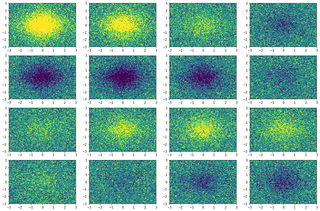
Figure 3. Snapshots state of the dynamical system.
Alright, now it is time to apply the DMD to the collected data. First,
we create a new DMD instance.
dmd = DMD(svd_rank=1, tlsq_rank=2, exact=True, opt=True)
We note there are four optional parameters:
- svd_rank: since the dynamic mode decomposition relies on
singular value decomposition, we can specify the number of the
largest singular values used to approximate the input data. It is
also possible to set it to 0 and the algorithm will calculate for
you the optimal rank truncation [6]. Moreover
it accepts non-integer values between 0 and
1, indicating the percentage of spectral energy you want to retain
with the truncation, for instance 0.8 means to retain at least 80%
of the cumulative energy of the singular values, starting from the
greatest.
- tlsq_rank: using the total least square, it is possible
to perform a linear regression in order to remove the noise on the
data; because this regression is based again on the singular value
decomposition, this parameter indicates how many singular values are
used.
- exact: boolean flag that allows to choose between the
exact modes or the projected one (see Subsection 6.1).
- opt: boolean flag that allows to choose between the standard
version and the optimized one. If true the optimal amplitudes of the
DMD modes are computed by minimizing the error between the time
evolution and all the original
snapshots [7]. If false the amplitudes are
computed using only the initial condition, that is the first
snapshot.
Then using a well known code design, borrowed from
scikit-learn [12, 1],
with the fit method it is possible to compute the DMD
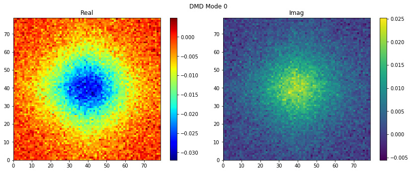
modes, given the original snapshots. Now we can plot the 2D modes
easily with plot_modes_2D, it is that simple!
dmd.fit(snapshots)

dmd.plot_modes_2D(figsize=(12,5))
We have everything to compute the reconstructed snapshots using the
DMD mode we have computed. The approximated system
is similar to the original one and, moreover, the noise is greatly
reduced.
fig = plt.figure(figsize=(18,12))

for id_subplot, snapshot in enumerate(dmd.reconstructed_data.T, start=1):


plt.subplot(4, 4, id_subplot)


plt.pcolor(x1grid, x2grid, snapshot.reshape(x1grid.shape).real, vmin=-1, vmax=1)
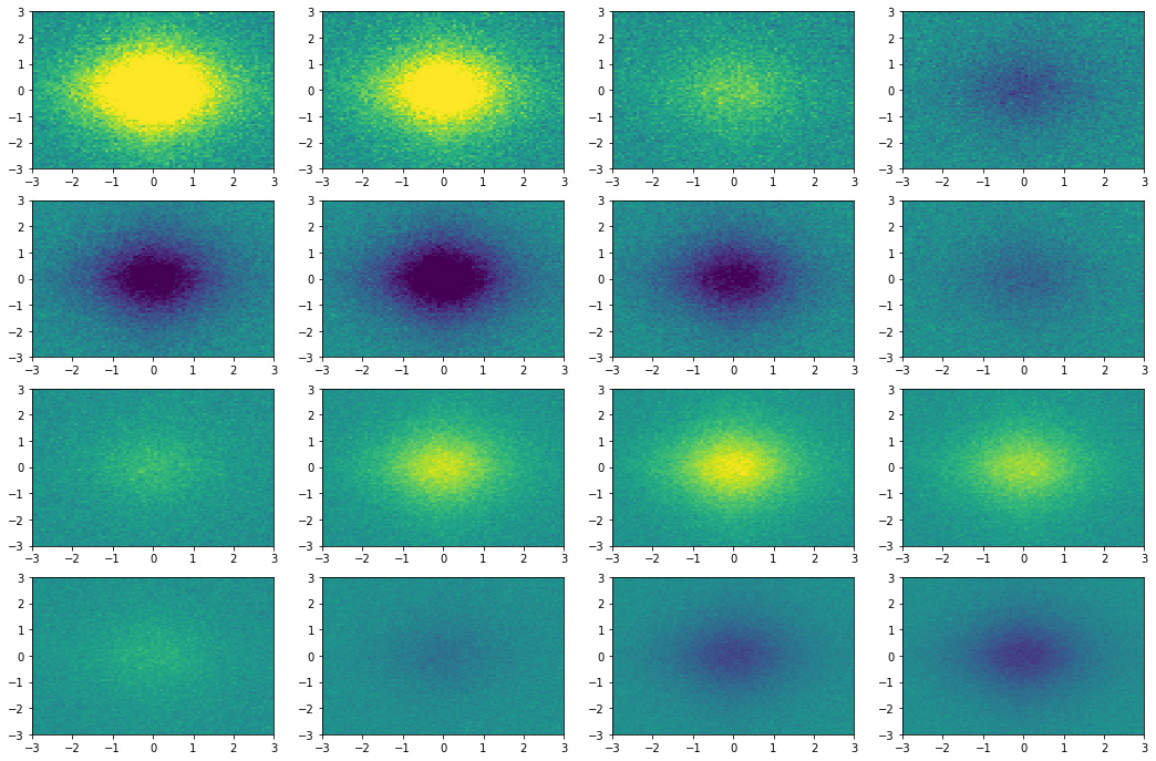
Figure 4. Snapshots state reconstructed by the DMD algorithm.
We can also manipulate the interval between the approximated states
and extend the temporal window where the data is reconstructed thanks
to DMD. Let us make the DMD delta time a quarter of the original and
extend the temporal window to \([0, 3t_{\text{org}}]\), where
\(t_{\text{org}}\) indicates the time when the last snapshot was
caught.
dmd.dmd_time['dt'] *= .25

dmd.dmd_time['tend'] *= 3
If we recalculate the reconstructed data with this new timeframe we obtain the video you can find at:
https://github.com/mathLab/PyDMD/blob/master/readme/dmd-example.gif.
6.4 DMD variants use cases
PyDMD allows to use many variants of the standard DMD
algorithm: the multi-resolution dynamic mode
decomposition (mrDMD), the forward/backward DMD, the DMD with control
(DMDc), the compressed DMD, and the high order dynamic mode
decomposition (HODMD). For all these implementations we refer to the
folder tutorials within the package repository, accessible at
https://github.com/mathLab/PyDMD/tree/master/pydmd, where there
is a tutorial for each one of them.
Acknowledgements
We thank the supervision of Professor Gianluigi Rozza, and the SISSA
mathLab group. The package was created in the framework of the project
HEaD, "Higher Education and Development", supported by Regione FVG ---
European Social Fund FSE 2014-2020, and under the European Union Funding for
Research and Innovation --- Horizon 2020 Program --- in the framework of
European Research Council Executive Agency: H2020 ERC CoG 2015
AROMA-CFD project 681447 "Advanced Reduced Order Methods with
Applications in Computational Fluid Dynamics" P.I. Gianluigi Rozza.
References
[1] L. Buitinck, G. Louppe, M. Blondel, F. Pedregosa, A. Mueller, O. Grisel, V. Niculae, P. Prettenhofer, A. Gramfort, J. Grobler, R. Layton, J. VanderPlas, A. Joly, B. Holt, and G. Varoquaux. API design for machine learning software: experiences from the scikit-learn project. In ECML PKDD Workshop: Languages for Data Mining and Machine Learning, 2013, pp. 108–122.
[2] N. Demo, M. Tezzele, G. Gustin, G. Lavini, and G. Rozza. Shape optimization by means of proper orthogonal decomposition and dynamic mode decomposition. In Technology and Science for the Ships of the Future: Proceedings of NAV 2018: 19th International Conference on Ship & Maritime Research, IOS Press, 2018, pp. 212–219.
[3] N. Demo, M. Tezzele, A. Mola, and G. Rozza. An efficient shape parametrisation by free-form deformation enhanced by active subspace for hull hydrodynamic ship design problems in open source environment. In The 28th International Ocean and Polar Engineering Conference, 2018.
[4] N. Demo, M. Tezzele, and G. Rozza. PyDMD: Python Dynamic Mode Decomposition. The Journal of Open Source Software, 3(22), 2018, p. 530.
[5] N. B. Erichson, S. L. Brunton, and J. N. Kutz. Compressed dynamic mode decomposition for background modeling. Journal of Real-Time Image Processing, 2016, pp. 1–14.
[6] M. Gavish and D. L. Donoho. The optimal hard threshold for singular values is 4/sqrt(3). IEEE Transactions on Information Theory, 60(8), 2014, pp. 5040–5053.
[7] M. R. Jovanovi{\'c}, P. J. Schmid, and J. W. Nichols. Sparsity-promoting dynamic mode decomposition. Physics of Fluids, 26(2), 2014, p. 024103.
[8] B. O. Koopman. Hamiltonian systems and transformation in hilbert space. Proceedings of the National Academy of Sciences, 17(5), 1931, pp. 315–318.
[9] J. N. Kutz, S. L. Brunton, B. W. Brunton, and J. L. Proctor. Dynamic mode decomposition: data-driven modeling of complex systems, volume 149, SIAM, 2016.
[10] J. N. Kutz, X. Fu, and S. L. Brunton. Multiresolution dynamic mode decomposition. SIAM Journal on Applied Dynamical Systems, 15(2), 2016, pp. 713–735.
[11] S. Le Clainche and J. M. Vega. Higher order dynamic mode decomposition. SIAM Journal on Applied Dynamical Systems, 16(2), 2017, pp. 882–925.
[12] F. Pedregosa, G. Varoquaux, A. Gramfort, V. Michel, B. Thirion, O. Grisel, M. Blondel, P. Prettenhofer, R. Weiss, V. Dubourg, J. Vanderplas, A. Passos, D. Cournapeau, M. Brucher, M. Perrot, and E. Duchesnay. Scikit-learn: Machine learning in {P}ython. Journal of Machine Learning Research, 12, 2011, pp. 2825–2830.
[13] J. L. Proctor, S. L. Brunton, and J. N. Kutz. Dynamic mode decomposition with control. SIAM Journal on Applied Dynamical Systems, 15(1), 2016, pp. 142–161.
[14] G. Rozza, M. H. Malik, N. Demo, M. Tezzele, M. Girfoglio, G. Stabile, and A. Mola. Advances in Reduced Order Methods for Parametric Industrial Problems in Computational Fluid Dynamics, ECCOMAS Proceedings, Glasgow, UK, 2018.
[15] P. J. Schmid. Dynamic mode decomposition of numerical and experimental data. Journal of fluid mechanics, 656, 2010, pp. 5–28.
[16] M. Tezzele, N. Demo, M. Gadalla, A. Mola, and G. Rozza. Model order reduction by means of active subspaces and dynamic mode decomposition for parametric hull shape design hydrodynamics. In Technology and Science for the Ships of the Future: Proceedings of NAV 2018: 19th International Conference on Ship & Maritime Research, IOS Press, 2018, pp. 569–576.
[17] M. Tezzele, N. Demo, A. Mola, and G. Rozza. An integrated data-driven computational pipeline with model order reduction for industrial and applied mathematics. Submitted, Special Volume ECMI, 2018.
| Model | |
| Software Type | |
| Language | |
| Platform | |
| Contact Person | |
| References to Papers | [1] L. Buitinck, G. Louppe, M. Blondel, F. Pedregosa, A. Mueller, O. Grisel, V. Niculae, P. Prettenhofer, A. Gramfort, J. Grobler, R. Layton, J. VanderPlas, A. Joly, B. Holt, and G. Varoquaux. API design for machine learning software: experiences from the scikit-learn project. In ECML PKDD Workshop: Languages for Data Mining and Machine Learning, 2013, pp. 108–122.
[2] N. Demo, M. Tezzele, G. Gustin, G. Lavini, and G. Rozza. Shape optimization by means of proper orthogonal decomposition and dynamic mode decomposition. In Technology and Science for the Ships of the Future: Proceedings of NAV 2018: 19th International Conference on Ship & Maritime Research, IOS Press, 2018, pp. 212–219.
[3] N. Demo, M. Tezzele, A. Mola, and G. Rozza. An efficient shape parametrisation by free-form deformation enhanced by active subspace for hull hydrodynamic ship design problems in open source environment. In The 28th International Ocean and Polar Engineering Conference, 2018.
[4] N. Demo, M. Tezzele, and G. Rozza. PyDMD: Python Dynamic Mode Decomposition. The Journal of Open Source Software, 3(22), 2018, p. 530.
[5] N. B. Erichson, S. L. Brunton, and J. N. Kutz. Compressed dynamic mode decomposition for background modeling. Journal of Real-Time Image Processing, 2016, pp. 1–14.
[6] M. Gavish and D. L. Donoho. The optimal hard threshold for singular values is 4/sqrt(3). IEEE Transactions on Information Theory, 60(8), 2014, pp. 5040–5053.
[7] M. R. Jovanovi{\'c}, P. J. Schmid, and J. W. Nichols. Sparsity-promoting dynamic mode decomposition. Physics of Fluids, 26(2), 2014, p. 024103.
[8] B. O. Koopman. Hamiltonian systems and transformation in hilbert space. Proceedings of the National Academy of Sciences, 17(5), 1931, pp. 315–318.
[9] J. N. Kutz, S. L. Brunton, B. W. Brunton, and J. L. Proctor. Dynamic mode decomposition: data-driven modeling of complex systems, volume 149, SIAM, 2016.
[10] J. N. Kutz, X. Fu, and S. L. Brunton. Multiresolution dynamic mode decomposition. SIAM Journal on Applied Dynamical Systems, 15(2), 2016, pp. 713–735.
[11] S. Le Clainche and J. M. Vega. Higher order dynamic mode decomposition. SIAM Journal on Applied Dynamical Systems, 16(2), 2017, pp. 882–925.
[12] F. Pedregosa, G. Varoquaux, A. Gramfort, V. Michel, B. Thirion, O. Grisel, M. Blondel, P. Prettenhofer, R. Weiss, V. Dubourg, J. Vanderplas, A. Passos, D. Cournapeau, M. Brucher, M. Perrot, and E. Duchesnay. Scikit-learn: Machine learning in {P}ython. Journal of Machine Learning Research, 12, 2011, pp. 2825–2830.
[13] J. L. Proctor, S. L. Brunton, and J. N. Kutz. Dynamic mode decomposition with control. SIAM Journal on Applied Dynamical Systems, 15(1), 2016, pp. 142–161.
[14] G. Rozza, M. H. Malik, N. Demo, M. Tezzele, M. Girfoglio, G. Stabile, and A. Mola. Advances in Reduced Order Methods for Parametric Industrial Problems in Computational Fluid Dynamics, ECCOMAS Proceedings, Glasgow, UK, 2018.
[15] P. J. Schmid. Dynamic mode decomposition of numerical and experimental data. Journal of fluid mechanics, 656, 2010, pp. 5–28.
[16] M. Tezzele, N. Demo, M. Gadalla, A. Mola, and G. Rozza. Model order reduction by means of active subspaces and dynamic mode decomposition for parametric hull shape design hydrodynamics. In Technology and Science for the Ships of the Future: Proceedings of NAV 2018: 19th International Conference on Ship & Maritime Research, IOS Press, 2018, pp. 569–576.
[17] M. Tezzele, N. Demo, A. Mola, and G. Rozza. An integrated data-driven computational pipeline with model order reduction for industrial and applied mathematics. Submitted, Special Volume ECMI, 2018. |