Gabriela Jaramillo, Department of Mathematics, University of Houston, 3551 Cullen Blvd., Houston, TX 77204-3008, USA. This work was supported by NSF DMS-1911742.

1. Introduction

Spiral waves appear in many physical and biological systems. We can see them in oscillating chemical reactions like the Belouzov-Zhabotinsky reaction as transient states in the aggregation of slime mold, and in heart and brain tissue. They capture our attention thanks to their visual appeal, but are also of interest because of their connection to anomalous heart conditions like tachycardia and cardiac fibrillation.

While spiral waves appear in both excitable and oscillatory media, our focus in this article will be on the latter. In particular, we consider systems whose dynamics undergo a Hopf bifurcation. The term oscillatory media then comes from the time oscillations that emerge, which also allow us to visualize these systems as a field of oscillating elements. When these elements are allowed to interact, either via a local form of coupling or through long range connections, spiral patterns and other coherent structures then form.

Here we concentrate on processes involving nonlocal interactions. An example of such systems is the following oscillating chemical reaction,

\( \begin{align*} \partial_t X(r,t) = &f(X,Y) + D(B-X)\\ \partial_t Y(r,t) = & g(X,Y)\\ \varepsilon \partial_t B(r,t) =& - B + d \Delta B + X , \end{align*} \)

which involves a fast component, \(B\), and nonlinearities, \(f(X,Y), g(X,Y)\) that support a limit cycle. In particular, by adiabatically eliminating the fast variable, (i.e., setting \(\varepsilon =0\) and solving for \(B = (\mathrm{I} - d\Delta)^{-1} X\),) one finds that these systems can be modeled using integro-differential equations of the form,

\( \begin{align*} \partial_t X(r,t) = &f(X,Y) + K\ast X\\ \partial_t Y(r,t) = & g(X,Y). \end{align*} \)

The convolution with the kernel \(K\) is then interpreted as a nonlocal form of diffusion.

Notice that when the range of nonlocal interactions is short, the convolution term is still well approximated by the Laplace operator. However, when this approximation breaks down, interesting patterns can emerge. Indeed, using numerical simulations Kuramoto showed that nonlocal interactions are in fact responsible for creating new patterns called spiral chimeras [11]. These patterns resemble an archimedean spiral in the far field, but as shown in Figure 1, they have a core that is not oscillating in synchrony with the rest of the pattern. Understanding why and how these structures arise provides the motivation for studying spiral waves in oscillatory systems with nonlocal coupling. In the following sections we summarize an approach for proving the existence of these patterns, and numerically explore the role that nonlocal interactions play in shaping these structures.

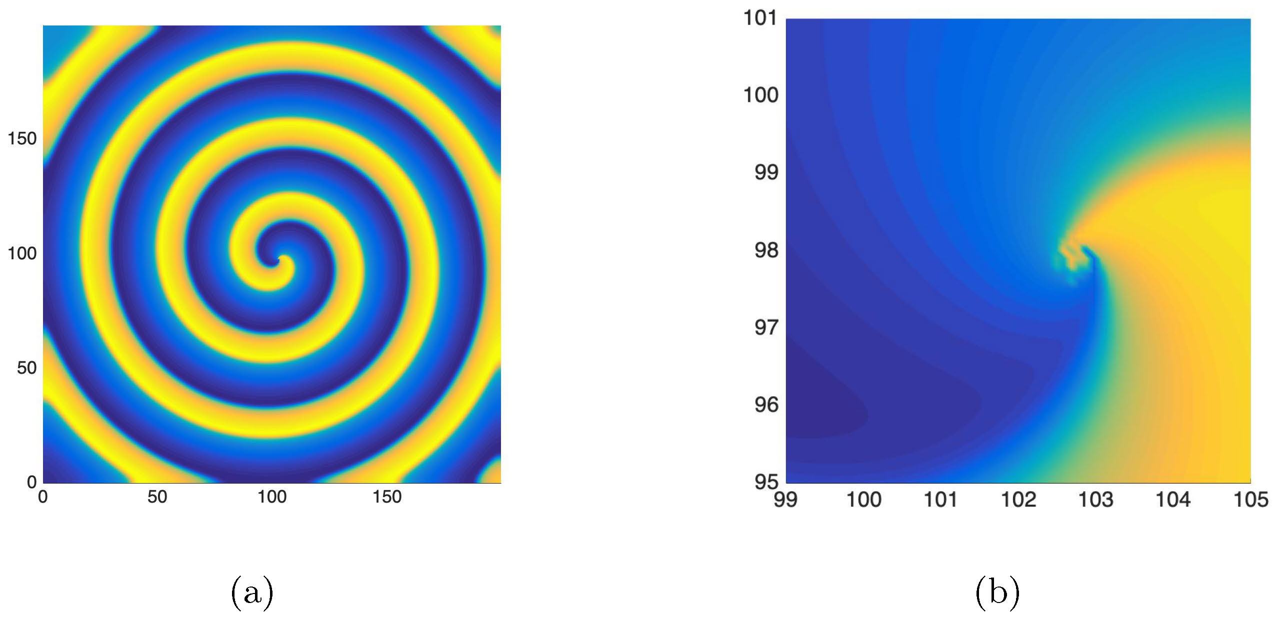
Figure 1: Example of a spiral chimera found by performing numerical simulations of the Fitz-Hugh Nagumo system appearing in [11]. The figure on the right zooms in into the core of the spiral appearing on the left.

Outline: In Section 2 we set up the notation and present results from numerical experiments that connect properties of the nonlocal coupling to the geometry of the spiral pattern. Then in Sections 3 and 4 we outline an approach for proving existence of these structures based on methods from functional analysis. Finally, in Section 5 we conclude with some open questions and an outlook of future directions.

2. A Simple Model

To maintain some level of generality, consider the following abstract integro-differential equation,

\( U_t = K \ast U + F(U;\lambda) \quad U \in \mathbb{R}^2 \quad x= (r,\theta) \in \mathbb{R}^2, \quad \lambda \in \mathbb{R}, \)

(1)

with nonlinearities, \(F(U;\lambda)\) that undergo a Hopf bifurcation when \(\lambda =0\), and nonlocal interactions modeled by the convolution operator \(K \ast\). For simplicity, suppose as well that the function \(K\) is of the same type as those used by Kuramoto to generate spiral chimeras. Therefore, \(K\) has Fourier symbol

\( \hat{K}( \xi ) = - \frac{ \sigma |\xi| ^2}{ ( 1 +D |\xi|^2)}, \qquad \mbox{with} \quad \xi \in \mathbb{R}^2, \quad \sigma, D>0. \)

(2)

Although this represents a specific form of nonlocal coupling, the analysis presented in the next sections can easily be extended to other functions, so long as their Fourier symbols are radially symmetric, uniformly bounded, and have a quadratic tangency near to origin. See [5] for more details on the assumptions governing the kernels \(K\).

One advantage of considering kernels of the form (2) is that one can then use numerical simulations to track how properties of the nonlocal operator affect the shape of the spiral pattern. For example, consider the following FitzHugh-Nagumo system

\( \begin{align} u_t & = K\ast u + \tau (u-u^3 -v)\\ v_t & = (\beta u + \delta), \end{align} \)

(3)

with parameters \(\delta = 0.2 , \beta = 1, \tau =0.1\), and \(K\) defined as above. In Figures 2 and 3 we simulate this system using an implicit spectral method [1] and a grid of length \(L=100\) with \(N=1024\) nodes. To enforce Neumann boundary conditions we employ the cosine Fourier transform.

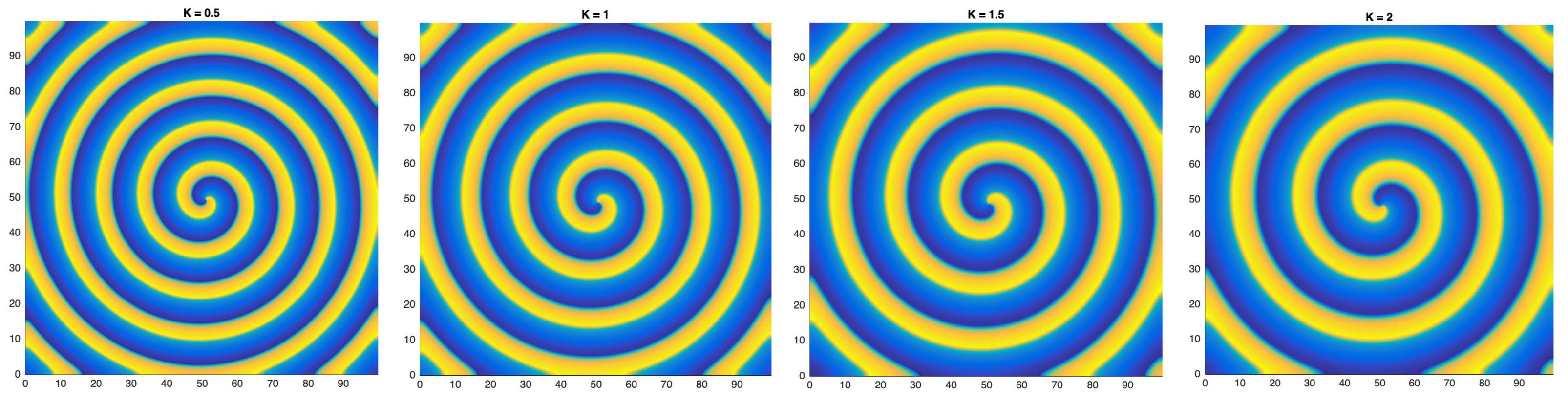
Figure 2: Numerical simulations of Fitz-Hugh Nagumo system in [11], using the kernel (2). Figures a) \(\sigma = 0.5\), b) \(\sigma =1.0\), c) \(\sigma =1.5\), d) \(\sigma =2.0\).

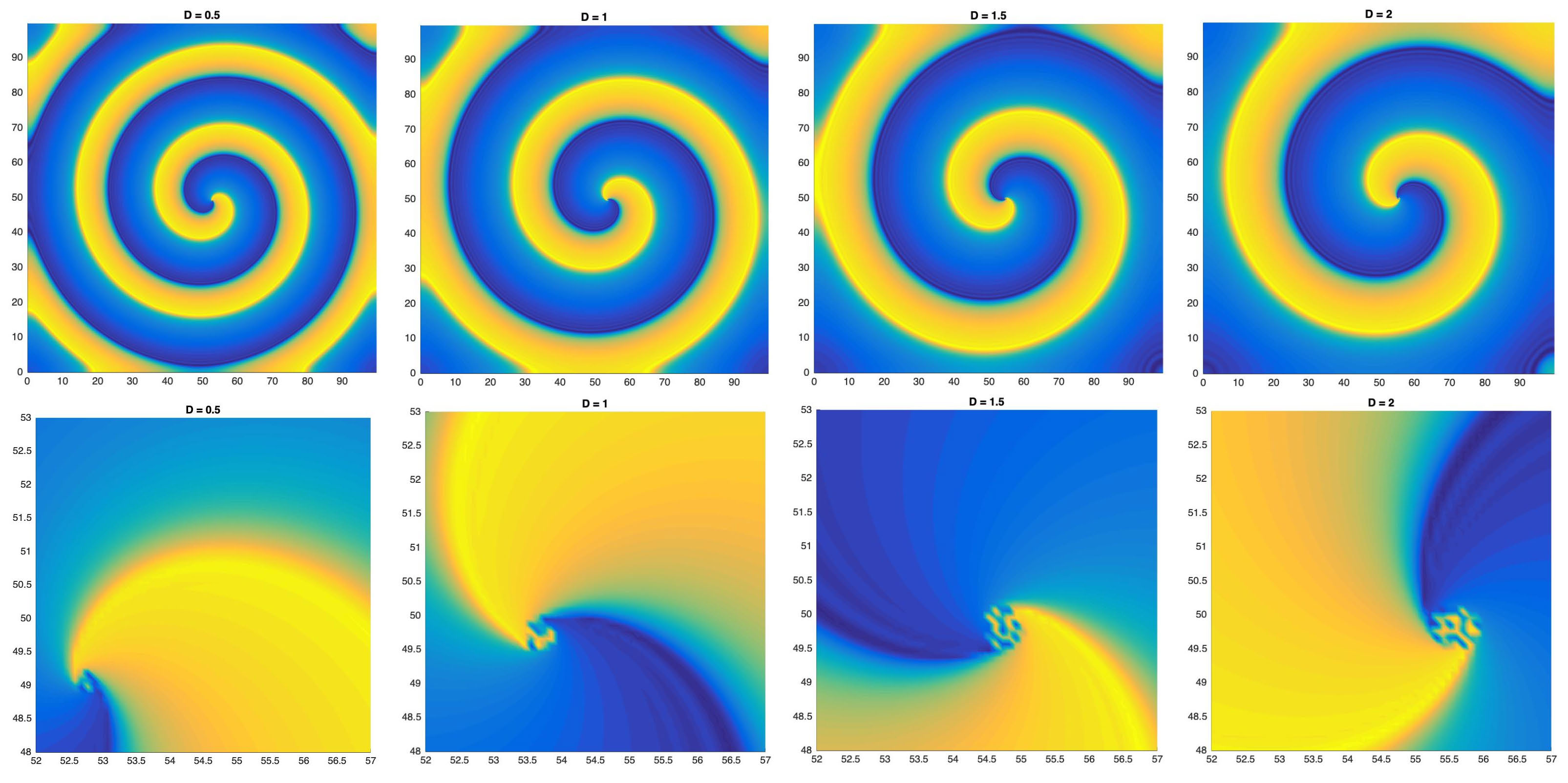
Figure 3: Numerical simulations of Fitz-Hugh Nagumo system in [11], using the kernel (2). Figures a) \(D = 0.5\), b) \(D =1.0\), c) \(D =1.5\), d) \(D =2.0\).

The figures show how by increasing the diffusivity constant, \(\sigma\), or the radius of nonlocal interactions, \(D\), one can reduce the spiral's wavenumber. n addition, notice how increasing the value of the parameter \(D\) leads to the formation of spiral chimeras.

One can heuristically explain the changes in the spiral's wavenumber and its core by looking at the shape of the Fourier symbol, \(\hat{K}\), as shown in Figure 4. The figure clarifies that the parameter \(\sigma\) controls the quadratic tangency of \(\hat{K}\) near the origin. As a result, increasing \(\sigma\) leads to Fourier symbols that are more narrow near the origin, which in turn implies that the band of unstable wavenumbers that the pattern can select becomes much smaller. Similarly, the parameter \(D\) controls the uniform bound of \(\hat{K}\) and as \(D\) increases, the \(L^\infty\) norm of the Fourier symbol becomes much smaller. This suggests that the zero amplitude solution may become unstable against all wavenumbers. Because the amplitude of these spiral patterns tends to zero near the origin, this provides a possible explanation as to why these structures possess an asynchronous core.

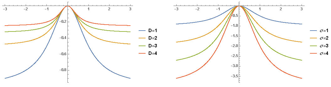
Figure 4: Plots of the Fourier symbol \(\hat{K}(|\xi|) = - \sigma |\xi| ^2/ ( 1 +D |\xi|^2)\), a) for different values of the parameter \(D\), and b) for different values of \(\sigma\).

One can confirm, at least formally, one of the above heuristic arguments. Indeed, the multiple-scale analysis outlined in Section 5 shows that one can use the following viscous eikonal equation

\( 0 = \Delta_{0} \phi_0 - b(\partial_S \phi_0)^2 + \Omega - \delta^2 b \tilde{g}, \)

(4)

to describe the phase dynamics of spiral waves. This equation is known to model the formation of target patterns in oscillatory media when an impurity is present, and was solved in [6] for the particular case of inhomogeneities, \(\tilde{g}\), that decay sufficiently fast at infinity. Since in the current context, target pattern solutions to the above equation also represent spiral wave solutions, one can borrow from these results.

Here it is important to point out that equation (4) represents a nonlinear eigenvalue problem. Both the function \(\phi_0\) and the constant \(\Omega\) are unknown. Target patterns are constructed by matching far field and intermediate approximations, and through this matching one is able to obtain approximations for the wavenumber \(k \sim \nabla \phi\) and the frequency \(\Omega = k^2\) of the pattern. In the case of spiral waves one finds that for sufficiently large values of the diffusivity constant \(\sigma\), the wave number is given by

\( k \sim C \exp({-1/M}), \qquad M \sim \left( \frac{\varepsilon^2 D \nu_I}{\sigma- \varepsilon^2 D \nu_R } \right)^2 \delta^2 \)

where \(\varepsilon\) represents the amplitude of the oscillations that emerge from the Hopf bifurcation, and the parameter \(\nu= \nu_R + \mathrm{i} \nu_I\) encodes information related to the linear part of the reaction terms \(F(U;\lambda)\). Notice that this approximation matches the results of the simulation. In particular, we can check that fixing the value of \(D\) and increasing the parameter \(\sigma\) results in a smaller wavenumber, \(k\).

We do want to emphasize that the above approximations are at this point formal. There is still work to be done to prove existence of spiral waves in these systems, and thus confirm that the formulas above provide indeed the correct expansions for the wavenumber. In the next sections we highlight some previous, current and future work in this direction.

3. Existence of Spiral Waves: Normal Form

To prove the existence of spiral patterns in oscillatory media with nonlocal diffusion, one proceeds in a similar manner as in the case of reaction diffusion systems. That is, one first derives an amplitude equation governing the dynamics of these structures, and then shows the existence of spiral wave solutions using this reduced equation. In the case of reaction diffusion systems it is possible to use tools from spatial dynamics, like center manifold theory and singular perturbation techniques, to carry out this program, see [9]. However, since in the present case the model equations are integro-differential equations, these tools are no longer available. In what follows we briefly summarize an alternative approach to derive the amplitude equation based on methods from functional analysis. Then, in Section 4 we outline how one can then find spiral wave solutions using this reduced equation.

The first step is to take advantage of the rotational symmetry of the pattern, and to look for general solutions of the form \(U(r, \theta) = U(r, \vartheta + ct)\), that are also periodic in the second argument. Notice that the symbol \(c\) represents the rotational speed of the wave, and is a parameter that needs to be determined along with the solution \(U\). Inserting this ansatz into equation (1) then leads to the following steady state system,

\( 0 = K \ast U - c \partial_\theta U+ F(U;\lambda). \)

One can now follow the approach taken in the physics literature and use multiple-scales to derive an amplitude equation. As it stands this method is formal, since it assumes that the solution can be expanded in powers of \(\varepsilon\sim \sqrt{\lambda}\). As a result, one then needs to show that this expansion converges, or equivalently, that the amplitude equation provides valid approximations to the solutions of the original system (1), see for example [12, 10]. However, because spiral wave solutions are periodic in time, it is possible to combine these two steps using a similar method to Lyapunov-Schmidt reduction.

Very briefly, the approach consists on carrying out the standard multiple-scale analysis giving us a hierarchy of equations at different powers of \(\varepsilon\). As usual, the first and second order equations can easily be solved. However, in contrast to the traditional method where one derives the amplitude equation at cubic order as a solvability condition, here all cubic and higher order terms are gathered into one equation. Then, as described in [5], by picking appropriate weighted Sobolev spaces and a suitable projection, it is possible to use Lyapunov-Schmidt reduction to split this equation into a solvable system, which has a linear operator that is invertible, and a reduced equation.

To see why this holds, use the Fourier transform in the angular variable, \(\theta\), to decompose the steady state equation as

\( 0 = \sum_{n \in \mathbb{Z}} ( K_n \ast U_n + B_n U_n + \tilde{F}_n(U;\lambda) ) \mathrm{e}^{\mathrm{i} n \theta}. \)

In this expression, the matrix \(B_n\) accounts for the operator \(-c \partial_\theta\) and the linear part of the reaction terms \(F(U;\lambda)\). In particular, \(B_n\) has eigenvalues \(- ( cn \pm i \omega)\), where \(\omega\) is the frequency of the time oscillations emerging from the Hopf bifurcation. As a result, if we pick \(c = c^* + \varepsilon^2 \mu\), where \(c^*n_0 = \omega\) for some integer \(n_0\) and \(\mu\) is to be determined, then \(B_{n_0}\) has a zero eigenvalue. This then leads us to decomposing the linear part of our equation into an invertible part, all those \(K_n \ast \; + B_n\) with \(n \neq n_0\), and a bounded part, \(K_{n_0} \ast\).

The reduced equation that is obtained from the above analysis then becomes the amplitude equation,

\( K_{\varepsilon,n_0} \ast w + \nu w + \alpha |w|^2 w + \mathrm{O}(\varepsilon |w|^4 w)=0, \)

(5)

where the convolution kernel \(K_{\varepsilon}\) represents a rescaling of \(K\) and has Fourier symbol \(\hat{K}_\varepsilon(\xi) = -\sigma|\xi|^2/(1 + \varepsilon^2 D |\xi|^2)\). The subscript \(n_0\) indicates that we are looking at the action of this operator in the direction of \(\mathrm{e}^{\mathrm{i} n_0 \theta}\). The imaginary part of \(\nu\) is related to the rotational speed of the wave, \(\mu\), and is a free parameter that needs to be determined when solving the equation. Finally, the constant \(\alpha\) encodes information about the nonlinear part of the reaction terms, \(F(U;\lambda)\).

It is important to emphasize that this amplitude equation is not a truncation. In fact, the equation involves all higher order terms. As a result, if one shows existence of solutions to equation (6), one immediately obtains existence of solutions to the full system (1). As expected, solving the reduced system is not a trivial matter. We give some insights into the issues that arise in the next section.

4. Existence of Spiral Waves: Current Work

Having derived equation (5) as a reduced system for our model (1), we now outline a path for proving the existence of spiral wave solutions. Because the convolution kernel \(K_{\varepsilon}\) has Fourier symbol

\( \hat{K}_{\varepsilon}( \xi) = - \frac{\sigma |\xi |^2}{ 1+ \varepsilon^2 D |\xi|^2}, \)

this task is simplified if we precondition the reduced system (5) with the operator \((1- \varepsilon^2 D \Delta)\). The result is an equation that resembles the complex Ginzburg-Landau equation (cGL),

\( \beta \left( \partial_{rr}w+ \dfrac{1}{r} \partial_rw - \dfrac{n^2}{r^2}\right) w + \nu w + \alpha |w|^2 w + \tilde{N} (w, \varepsilon)=0, \)

where \(\beta = (\sigma -\varepsilon^2 D \nu_R) - \mathrm{i} (\varepsilon^2 D \nu_I).\) Notice how even though the linear operator in the equation above is no longer a nonlocal operator, the main features of the convolution kernel \(K\) are still encoded in the constant \(\beta\).

To find spiral wave patterns one can then proceed with a multiple-scale analysis using the same scalings that are typical for deriving the phase dynamics approximation of the cGL, see [2]. This leads to a hierarchy of equations at different powers of a small parameter \(\delta\). The order \(\mathrm{O}(1)\) system encapsulates information about the amplitude of the pattern, while the order \(\mathrm{O}(\delta^2)\) system describes the dynamics of the phase. As when deriving the amplitude equation, the remaining terms can then be summarized as one system of equations. The objective is then to pick correct Sobolev spaces, so that one may apply Lyapunov-Schmidt reduction, thus closing the argument and proving the existence of solutions. We close this section summarizing some of the questions that arise in this approach.

The order \(\mathrm{O}(1)\) terms: These terms give us the following system of equations for the amplitude, \(\rho_0\), of the spiral pattern,

\( \begin{align} 0 = & \beta_R \Delta_1\rho_0 + \nu_R \rho_0 - \nu_R \rho_0^3,\\ 0 = & \beta_I \Delta_1 \rho_0 - \tilde{\alpha}_I \rho_0 + \tilde{\alpha}_I \rho_0^3. \end{align} \)

(6)

Notice in particular that when \(\beta_R, \nu_R >0\) the first equation also models the amplitude of spirals arising in \(\lambda-\omega\) systems. These systems, which include more general nonlinearities that the ones appearing in (6), are known to model oscillatory media, see [4, 3, 8]. The general case was studied by Kopell and Howard in [8], who proved the existence of positive solutions \(\rho_0\). In particular, they showed that when \(\nu_R =1\), these solutions approach the constant \(1\) in the far field.

Because the system is redundant, once the first equation is solved the remaining terms can be written as a single function \(g \sim (1- \rho_0^2)\rho_0\), which is then pushed down to the order \(\mathrm{O}(\delta^2)\) system. As pointed out next, it then becomes important to know the decay rate of the function \(g/\rho_0\), or equivalently, to know how quickly the amplitude, \(\rho_0\), approaches its constant value at infinity. Numerically, it is possible to check that the term \(g/\rho_0\) is of order \(\mathrm{O}(1/r^2)\) as \(r\) goes infinity (see Figure 5), but one would like to make this precise.

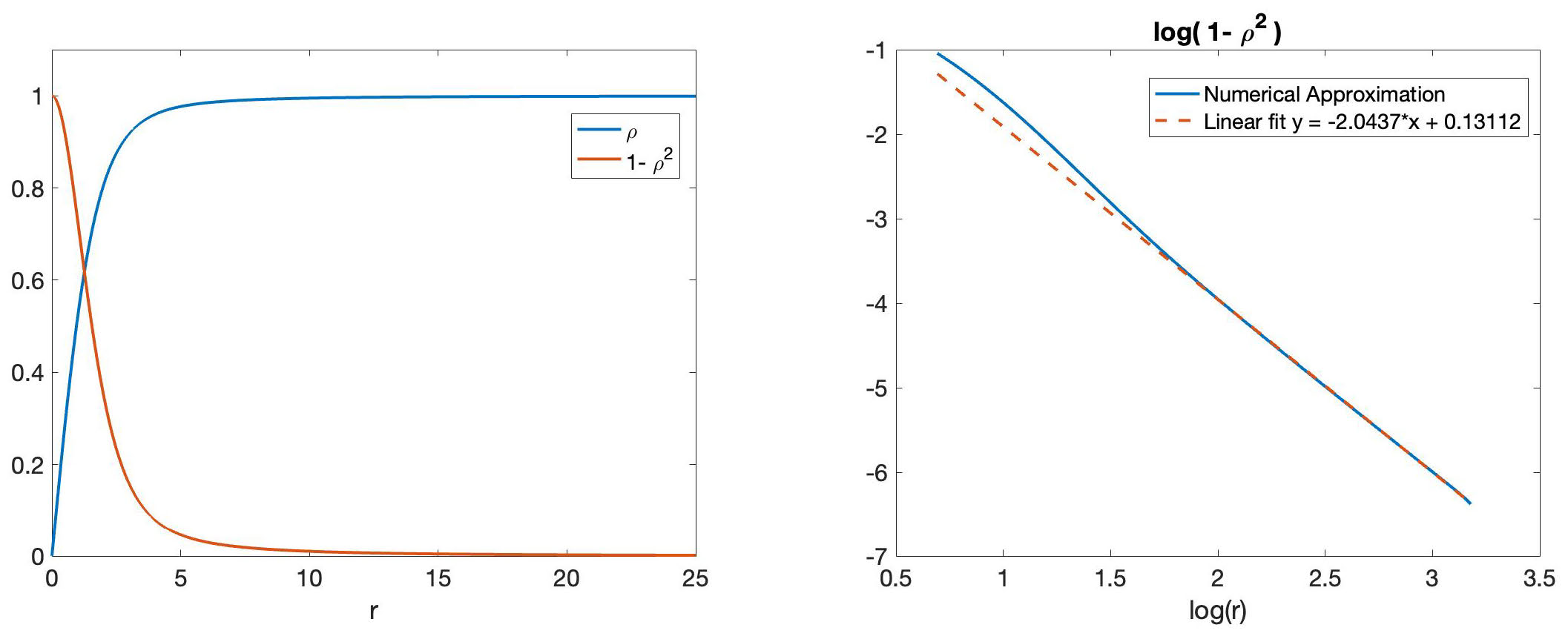
Figure 5: Numerical approximation of first equation in system (6), with \(\nu_R= \beta_R =1\).

The order \(\mathrm{O}(\delta^2)\) terms: Not surprisingly, when gathering terms of order \(\mathrm{O}(\delta^2)\), one sees that the resulting system of equations can be reduced to the following viscous eikonal equation for the phase \(\phi_0\),

\( 0 = \Delta_{0} \phi_0 - b(\partial_S \phi_0)^2 + \Omega - \delta^2 b g/ \rho_0. \)

(7)

Here \(b\) is a constant, \(\Omega\) is a parameter involving the unknown \(\nu_I\), and the function \(g\), as explained above, is an inhomogeneity that is a function of \(\rho_0\).

As mentioned in Section 3, equation (7) is known to provide a model for the emergence of target patterns in oscillatory media, and has been solved in the case of inhomogeneities that decay at order \(\mathrm{O}(1/r^{2+ \delta})\) with \(\delta>0\), see [6]. However, as depicted in Figure 5, the function \(g/\rho_0 \sim (1 - \rho_0^2)\) decays only at order \(\mathrm{O}(1/r^{2})\). Thus, equation (7) represents a border case that has not been solved before. Nonetheless, the numerical results presented in Figure 6 show that solutions to this equation do exist, even for inhomogeneities that decay slower than \(1/r^2\). Proving existence of target patterns for these extreme cases is part of our current efforts.

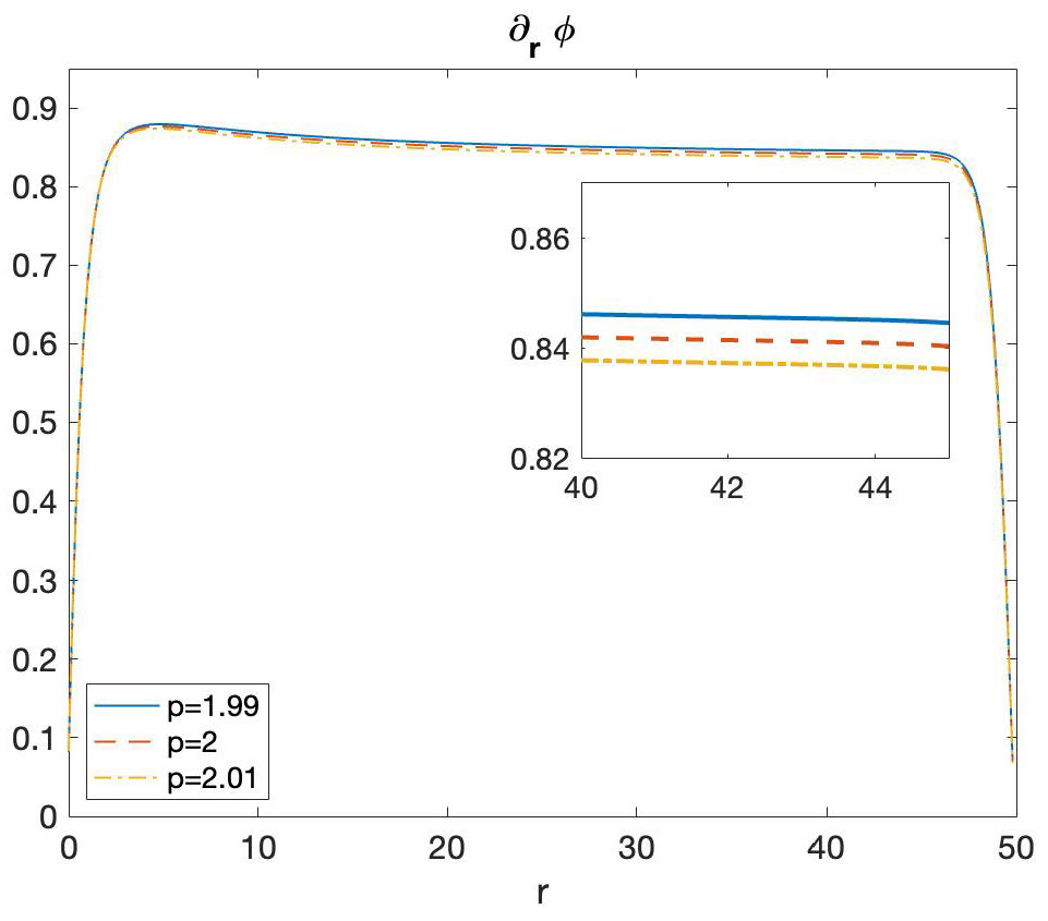
Figure 6: Numerical simulation of the eikonal equation \(\partial_t \Phi = \Delta \Phi - | \nabla \Phi|^2 +g\) for different inhomogeneities \(g=-2.5/(1+r^2)^{p/2}\) on a square domain. In this case, target patterns satisfy \(\Phi(r,t) = \phi(r) - \Omega t\). The figure depicts \(\partial_r \phi\). Time evolution uses a spectral method to discretize the space variable and an RK-4 method for the time stepping, [7]. Parameters: length \(L=100\), number of nodes \(N=512\), time stepping \(dt = 0.5\).

Higher order terms: The remaining terms from the multiple-scale analysis can be gathered as a system of equations in the variables \(R_1, \phi_1\)

\( \begin{align*} 0 = & \nu_R ( 1- 3 \rho_0^2)R_1 - \beta_I \rho_0 \Delta_{0} \phi_1 -2 \beta_R \rho_0 \partial_r \phi_0 \partial_r \phi_1 + N_1(R_1, \phi_1;\delta),\\ 0 = & \tilde{\alpha}_I( 3 \rho_0^2 -1)R_1 + \beta_R \rho_0 \Delta_{0} \phi_1 -2 \beta_I \rho_0 \partial_r \phi_0 \partial_r \phi_1 + N_2(R_1, \phi_1; \delta). \end{align*} \)

To close the argument and prove existence of spiral waves, one would now like to apply Lyapunov-Schmidt reduction to the above system and find solutions that bifurcate from \((R1,\phi_1;\delta) =(0,0;0)\). This requires that the linear part of the equations define a Fredholm operator, and is one of the main challenges in this problem.

To see where the difficulties lie, notice first that linearization includes the operator

\( \mathcal{L}\phi_1= \Delta_{0} \phi_1 - \partial_r \phi_1. \)

which has a zero eigenvalue embedded in its essential spectrum. As a result this operator does not have a closed range and it is therefore not a Fredholm operator when acting as a map between standard Sobolev spaces.

While this issue can be resolved if we use instead Sobolev spaces that impose some level of algebraic decay or growth on functions (see [6]), this comes at cost. Indeed, because the function \(\rho_0\) appears in the nonlinearities and is uniformly bounded, one needs to use spaces that allow for algebraic growth. However, these spaces are no longer Banach algebras, so that the nonlinear terms are not well defined in this case.

Therefore, finding solutions to the above system requires that we pick Banach spaces that provide a balance between Fredholm properties and well defined nonlinearities. Possible candidates include spaces that separate the near field and far field behavior of the solution. This allows one to construct first order approximations that account for the far field behavior, which in the case of spiral waves is described by \(L^\infty\) functions, while any higher order corrections are restricted to the core of the pattern and are viewed as algebraically localized functions. For example we may take \(X = H^2_\gamma(\mathbb{R}^2) \oplus W^{2, \infty}(\mathbb{R}^2)\), where the subscript \(\gamma\) informs us about the level of algebraic decay.

5. Outlook

We close with two open questions and a couple of future directions.

1. When the parameter \(\sigma\) is large we are able to find a formal expansion for the spiral's wavenumber. This expansion is obtained, in part, by solving the first equation in system (6). This equation is solvable because the parameter \(\beta_R\) is positive whenever \(\sigma\) is sufficiently large. What happens then if \(\sigma\) is smaller than the coupling radius, and the parameter \(\beta_R\) is now negative? If one also assumes that the parameter \(\beta_I\) is positive and the parameter \(\tilde{\alpha}_I\) is negative, then the second equation in (6) can be solved. This would then give us a different expansion for the wavenumber, and the question is then whether this expansion can explain the behavior seen in Figure 3.
2. According to Figure 3, when \(\beta_r<0\) we are also in the situation when spiral chimeras are formed. The previous item suggest that we should be able to proof the existence of these patterns using the approach outlined in Section 4. However, because this method approximates the solution in the far field, but summarize its behavior near the core as a function with algebraic decay, it is not possible to distinguish between both patterns just by looking at the form of the solution. How can we then re-gain information about the spiral's core?
3. More broadly, after proving the existence of spiral waves, how do we then proceed to study their stability?
4. And finally, can the above methods, which are based on functional analysis, be used to understand other two or three dimensional patterns?

References

[1]   A. Bueno-Orovio, D. Kay, and K. Burrage, Fourier spectral methods for fractional-in-space reaction-diffusion equations, BIT Numerical Mathematics, 54 (2014), pp. 937–954.

[2]   A. Doelman, B. Sandstede, A. Scheel, and G. Schneider, The dynamics of modulated wave trains, American Mathematical Soc., 2009.

[3]   J. Greenberg, Spiral waves for \(\lambda\)-\(\omega\) systems, II, Advances in Applied Mathematics, 2 (1981), pp. 450–455.

[4]   J. M. Greenberg, Spiral waves for \(\lambda\)-\(\omega\) systems, SIAM Journal on Applied Mathematics, 39 (1980), pp. 301–309.

[5]   G. Jaramillo, Rotating spirals in oscillatory media with nonlocal interactions and their normal form, Discrete and Continuous Dynamical Systems - S, 0 (2022).

[6]   G. Jaramillo and S. C. Venkataramani, Target patterns in a 2d array of oscillators with nonlocal coupling, Nonlinearity, 31 (2018), p. 4162.

[7]   A. Kassam and L. Trefethen, Fourth-Order time-stepping for stiff PDEs, SIAM Journal on Scientific Computing, 26 (2005), pp. 1214–1233.

[8]   N. Kopell and L. Howard, Target pattern and spiral solutions to reaction-diffusion equations with more than one space dimension, Advances in Applied Mathematics, 2 (1981), pp. 417–449.

[9]   A. Scheel, Bifurcation to spiral waves in reaction-diffusion systems, SIAM Journal on Mathematical Analysis, 29 (1998), pp. 1399–1418.

[10]   G. Schneider, The validity of generalized Ginzburg-Landau equations, Mathematical Methods in the Applied Sciences, 19 (1996), pp. 717–736.

[11]   S.-i. Shima and Y. Kuramoto, Rotating spiral waves with phase-randomized core in nonlocally coupled oscillators, Phys. Rev. E, 69 (2004), p. 036213.

[12]   A. van Harten, On the validity of the Ginzburg-Landau equation, Journal of Nonlinear Science, 1 (1991), pp. 397–422.