Rachel Nicks, School of Mathematical Sciences, University of Nottingham, Nottingham, NG7 2RD, UK.

1. Introduction

You are most likely aware that illusions or hallucinations can occur in response to viewing certain images. For example, illusory movement can be perceived within a static image such as rotating snakes [5] (see Fig. 1 and for further examples visit [10]) or the flickering wheel illusion where the static wheel with 30-40 spokes, is experienced as flickering when viewed in the visual periphery [25]. It is also known that relatively simple patterns of regular stimuli, such as radial lines or concentric rings, are enough to induce illusory motion at right angles to those of the stimulus pattern [13]; a phenomenon known as the MacKay effect. An image of high density rays which can induce the MacKay effect is shown in Fig. 2. The tools of psychophysics and mathematical models of large-scale neural activity in primary visual cortex (V1) can be used to shed light on possible origins of such phenomena.

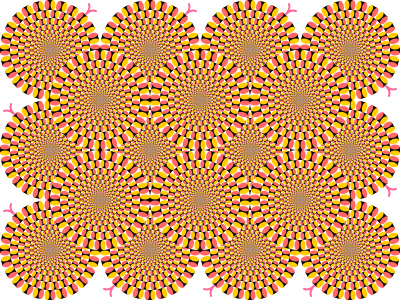
Figure 1: A static image inducing illusory movement: An example of a peripheral drift illusion known as rotating snakes (Image credit: Cmglee, CC BY-SA 3.0, via Wikimedia Commons).

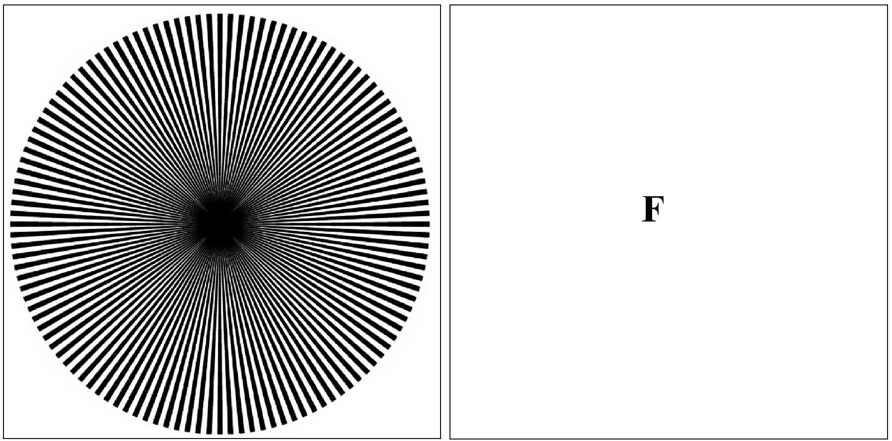
Figure 2: MacKay ray figure which induces hallucinatory effects orthogonal to the input. Fixate for ten seconds on the center of the figure, then transfer gaze to the blank fixation (F) and notice the streaming circular effects in the blank area, roughly orthogonal to the orientation of the rays. (Image credit: Fig. 1 of [26] see Source, CC BY 2.5, via Wikimedia Commons).

Visual cortex is active even in the absence of retinal stimulation. Hallucinations of geometric patterns can be induced through ingestion of drugs, placing deep pressure on the eyeballs or in response to flickering lights [11, 22]. These hallucinations often take the form of lattice (a.k.a. honeycomb, grating, or chessboard), cobweb-like, tunnel (a.k.a. funnel, cone or vessel), and spiral patterns. When transformed from the retinocentric (polar) coordinates of the eye to the (cartesian) coordinates of V1, these so-called Klüver form constants manifest as simple geometric planforms such as rolls, hexagons, squares, etc. [23]. The seminal work of Ermentrout and Cowan in the late 1970s [8], and the inclusion of the dynamics of orientation selective cells in the later work of Bressloff et al. [4], demonstrate that spontaneous pattern formation in simple integro-differential equation models of visual cortex can be used to explain drug induced geometric visual hallucinations by generating representatives of the Klüver form constants. The models studied by Ermentrout and Cowan [8] and Bressloff et al. [4] are examples of neural field models which describe large scale dynamics of neural tissue [6], and in both cases the authors focus on the description of cortical activity patterns which occur spontaneously; that is, patterns that are induced via a Turing instability occurring upon variation of parameters intrinsic to the model.

To understand the mechanisms for sensory induced hallucinations in response to external drive (presentation of an image to the retina) we must consider how the drive interacts with the self-organised activity patterns in V1. This was recognised by the psychophysicists Billock and Tsou, who tried to induce certain geometric hallucinations by biasing them with an appropriate visual stimuli from a flickering monitor [3]. For example, a set of centrally presented concentric rings was expected to induce a hallucination of further circles in the surround. Instead, and perhaps surprisingly, they found that fan-shaped patterns were perceived in the surround (and a complementary pattern of concentric rings in the surround for radial patterns in the centre). Moreover, the hallucinatory fan patterns were observed to rotate at about 1 revolution per second (with direction of rotation arbitrary and subject to reversal). Their findings are summarised in Fig. 3. The retino-cortical map away from the fovea can be approximated by a quasi-conformal dipole map [2] which maps a point \((r, \theta)\) in the polar coordinates of the retina to the point \((x,y) = (\ln (r), \theta)\) in the cartesian coordinates of V1. This tells us that the corresponding patterns of neural activity in the primary visual cortex for rings and arms in the retina are orthogonal stripe patterns and that spiral arms in retinal coordinates would map to oblique stripes in cortical coordinates, as illustrated in Fig. 4. The implication of the psychophysical experiments of Billock and Tsou is that cortical forcing by spatially periodic input can excite orthogonal modes of neural activity, and furthermore the forcing can induce hallucinatory motion.

A natural question arises as to whether there are minimal models of visual cortex with external drive capable of supporting the observed phenomena of orthogonal response and pattern movement, and do they require a departure from existing neural field models. In short, the answer is that standard neural field models with a state-dependent drive are sufficient as has been shown by Nicks et al. [19]. This article briefly summarises the work in [19], demonstrating that techniques originally developed for analysing spatially forced partial differential equation models [15] can be adapted to nonlocal neural field models, and that these can be used to uncover the parameter windows that robustly reproduce orthogonal responses to spatially periodic forcing. In doing so this highlights the potential mechanisms that can underpin the original psychophysical observations of Billock and Tsou.

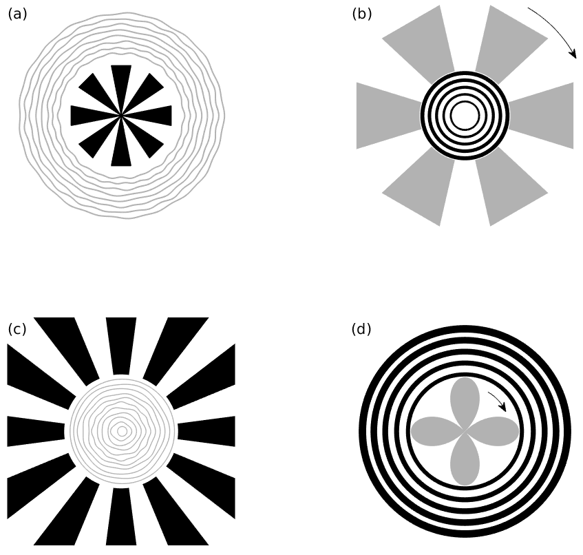
Figure 3: An illustration of the biasing stimuli (black) and hallucinatory percepts (grey) as reported by Billock and Tsou and redrawn from [3]. (a) If the area around a small fan shape is flickered, subjects report seeing illusory circular patterns, (b) if the area around a circular pattern is flickered, an illusory rotating fan shape is perceived, (c) if a biasing pattern of peripheral radial arms is presented then central rings are perceived, and (d) a rotating petal-like pattern often appears in the flickering central area in response to a peripheral set of biasing concentric rings. The arrows indicate perceived rotation.

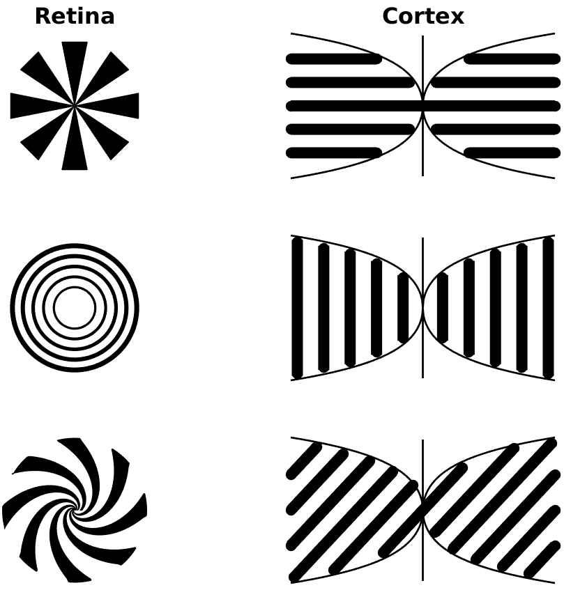
Figure 4: An illustration of the retino-cortical map that takes points of stimuli on the retina to points in V1 (left and right primary visual cortex), showing how radial arms, rings, and spirals on the retina transform to oriented stripes on V1.

2. A model with a mechanism for orthogonal response to forcing

Given the success of neural field models in describing drug-induced (spontaneous) hallucinations in V1, it is natural to see if they are also capable of explaining the opponency in visual hallucinatory phenomena. We therefore consider a minimal model of the evolution of synaptic activity in V1 as an effective single population and include a forcing term to mimic sensory input to the system. Adopting a planar model for V1, neural activity at a point \(\mathbf{r} =(x,y) \in \mathbb{R}^2\) is represented by the scalar field \(u(\mathbf{r}, t)\) whose dynamics are given by

\( \frac{\partial}{\partial t}u(\mathbf{r}, t) = -u(\mathbf{r}, t) + \int_{\mathbb{R}^2} w(\mathbf{r}- \mathbf{r}') f(u(\mathbf{r}',t); \mu)\, \mbox{d} \mathbf{r}' + \gamma u(\mathbf{r}, t) I(\mathbf{r}, t), \)

(1)

where the nonlinear firing rate \(f\) is chosen as a sigmoid with a threshold \(h\) and steepness \(\mu\) at threshold:

\( f(u; \mu, h) = \frac{1}{1 + \mathrm{e}^{-\mu(u - h)}}. \)

(2)

Here we set \(h=0\) and write \(f(u; \mu, 0) = f(u; \mu)\) but note that cases where \(h\neq 0\) are treated in [19].

The different effects of excitatory and inhibitory interactions between points in the tissue are encoded in a single kernel \(w\) whose sign indicates whether an interaction is excitatory (positive) or inhibitory (negative). For concreteness the kernel \(w\) is chosen as the rotationally symmetric Wizard hat function, \(w(\mathbf{r}) = w(r)\), where \(r=|\mathbf{r}|\) and

\( w(r) = A \mbox{e}^{-r/\sigma} - \mbox{e}^{-r}, \qquad A>1, \sigma<1. \)

(3)

This kernel describes a tissue with short-range excitation and long-range inhibition, which is well known for its pattern forming properties [1, 7]. The choice of kernel (3) with \(A= \sigma^{-2}\) satisfies the balance condition \(\int_{\mathbb{R}^2} \mbox{d} \mathbf{r} \, w(|\mathbf{r}|)= 0\) which places the homogeneous steady state of (1) at \(u=0\). The external input is described by \(I(\mathbf{r}, t)\) with the strength of the forcing being given by \(\gamma \in \mathbb{R}\). From a biological perspective cells in V1 would be driven by synaptic currents, and these in turn would be mediated by conductance changes arising from afferent inputs. These currents have a simple ohmic form that multiplies the voltage of the post-synaptic neuron with that of the conductance change. Thus the input signal is mixed with the state of the neuron. We allow for a simple form of mixing by including a multiplication of \(I\) with the state \(u\). For the specific choice of external input we take a simple static spatial pattern of stripes in the \(x\)-direction with wavenumber \(k_f\), \(I(\mathbf{r},t) = \cos(k_f x)\) (corresponding to concentric circles under the inverse retinocortical mapping) and recall that our interest is in the development of striped patterns in neural activity along the \(y\)-direction.

2.1. Patterning in the absence of drive

Linear stability analysis reveals that in the absence of drive (\(\gamma=0\)) the homogeneous steady state \(u=0\) of (1) undergoes a static Turing instability when

\( \frac{\mu_c}{4}= f'(0; \mu_c) = \frac{1}{\widehat{w}(k_0)}, \)

(4)

where, denoting \(|\mathbf{k}|=k\),

\( \widehat{w} (k) =\widehat{w} (\mathbf{k}) = \int_{\mathbb{R}^2} \mbox{d} \mathbf{r} \, w(\mathbf{r}) \mbox{e}^{- i \mathbf{k} \cdot \mathbf{r}}, \)

is the 2D Fourier transform of the connectivity kernel which has a local maximum at \(k_0 >0\). Beyond the Turing instability (\(\mu>\mu_c\)), we expect the emergence of patterns with spatial wavenumber \(k_0\). We are interested in the effects of structured external forcing with spatial wavenumber \(k_f\) on such patterns.

2.2. Resonant patterns in the presence of drive

The periodic forcing of pattern forming systems can lead to novel behaviours as well as frequency or wavenumber locking. The mathematical study of spatially forced systems is relatively underdeveloped compared to that of temporal forcing, with an exception being the work of Manor et al. [14]. In this and follow up work [15, 16, 17], these authors consider idealised pattern forming systems of Swift-Hohenberg type poised near Turing instability to a pattern with a wavenumber \(k_0\) with weak spatial periodic spatial forcing at wavenumber \(k_f\). They show that if \(k_f\) is close to \(2k_0\) then stable resonant stripes can be formed. Importantly, they also establish that if the mismatch between \(k_f\) and \(2k_0\) is high, then a locked pattern can still develop albeit with a wavevector component perpendicular to the forcing direction. Given that this is one of the major properties of the psychophysical experiments of Billock and Tsou that we are seeking to understand, it is natural to see if the corresponding phenomenon can arise in a neural field model.

Weakly nonlinear analysis can be used to derive amplitude equations for the emergent patterns in the neighbourhood of a Turing instability where we also include static external forcing \(I(\mathbf{r},t) = \cos(k_f x)\) with forcing strength \(\gamma\ll 1\). Beyond the Turing instability all wavevectors \(\mathbf{k}= (k_x, k_y)\) of magnitude \(|\mathbf{k}|=k_0\) emerge spontaneously. We investigate resonance with those which are locked to the forcing wavevector \((k_f,0)\). Here, \(n\):\(1\) resonant solutions have \(k_x = k_f/n = k_0 - v_2\) (see Fig. 5) where \(v_2\) is a mismatch parameter satisfying \(0\leq v_2\leq 2k_0\). Locking in the forcing direction creates a wavevector component in the orthogonal direction, \(k_y\), to compensate for the unfavourable forcing wavenumber, so that \(k_y = \sqrt{k_0^2 - k_x^2}\) to achieve the total wavenumber \(k_0\).

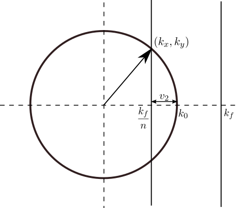
Figure 5: The circle indicates the ring of fastest growing wavenumbers with critical value \(|\mathbf{k}|=k_0\), for \(\mathbf{k}= (k_x, k_y)\). The forcing wavevector is \(\mathbf{k_f} = (k_f,0)\). We take \(k_x = k_f/n = k_0 - v_2\) for mismatch parameter \(v_2\), with \(n \in \mathbb{Z}\). The wavevector component \(k_y\) satisfies \(k_y^2 = k_0^2 - k_x^2\) to achieve the total wavenumber \(k_0\).

The structure of the two-dimensional patterns that form are, to leading order,

\( u \simeq A(\chi, \Upsilon, \tau) \mbox{e}^{i(k_x x + k_y y)} + B(\chi, \Upsilon, \tau) \mbox{e}^{i(k_x x - k_y y)} + \mbox{ c.c.} \)

(5)

where the complex amplitudes \(A(\chi, \Upsilon, \tau), B(\chi, \Upsilon, \tau)\) vary slowly in space and time (with the scaling \(\chi = \epsilon x\), \(\Upsilon = \epsilon y\), \(\tau= \epsilon^2 t\) for a small parameter \(\epsilon\)). Weakly nonlinear analysis provides the coupled system of Ginzburg-Landau equations satisfied by these amplitudes (see [19] for details of the calculations). Scaling back to the original time and space variables gives the two complex-valued coupled nonlinear ODEs that describe the evolution of the amplitudes \(a(x,y,t) = \epsilon A(\chi, \Upsilon, \tau)\), \(b(x,y,t)= \epsilon B(\chi, \Upsilon, \tau)\). The form of the amplitude equations depends on the value of \(n\) with certain terms only appearing when \(n=2\) and others only when \(n\neq 2\). Since orthogonal response is seen in the Swift-Hohenberg equation for the \(2\):\(1\) resonance [15] we also focus on the case where \(n=2\) and the amplitude equations are

\( \beta_c \frac{\partial a} {\partial t} = \epsilon^2 \delta a - \Phi_1|a|^2a -\Phi_2 |b|^2a - \frac{\beta_c^2}{2k_0^2}\widehat{w}^{\prime\prime}(k_0)\left(k_x\partial_{x} + k_y\partial_{y}\right)^2 a + \frac{\gamma \beta_c}{2} b^* , \)

(6)

\( \beta_c \frac{\partial b} {\partial t} = \epsilon^2 \delta b - \Phi_1|b|^2b -\Phi_2 |a|^2b - \frac{\beta_c^2}{2k_0^2}\widehat{w}^{\prime\prime}(k_0)\left(k_x\partial_{x} + k_y\partial_{y}\right)^2 b + \frac{\gamma \beta_c}{2} a^* , \)

(7)

where

\( \Phi_1 = -2\beta_2\zeta(k_0) - 3 \beta_3, \quad \Phi_2 = -2 \beta_2(\zeta(k_x) + \zeta(k_y)) - 6\beta_3, \quad \mbox{with} \ \ \zeta(k)= \frac{2 \beta_2 \widehat{w}(2k)}{1-\beta_c \widehat{w}(2k)}, \)

and \(\beta_j = f^{(j)}(0, \mu_c)\) are the Taylor coefficients of the firing rate. Note that \(\beta_1\) is treated as the bifurcation parameter: \(\beta_1 = \beta_c + \epsilon^2 \delta\) where \(\beta_c =f'(0, \mu_c)= \mu_c/4\). Furthermore, since we chose \(h=0\) in (2), \(\beta_2=0\) and \(\beta_3= -\mu_c^3/8\). Constant solutions of these equations correspond to \(2\):\(1\) resonant patterns which exist beyond the Turing instability. The amplitude equations support two types of spatially homogeneous, constant patterns; rectangles (with equal amplitudes, \(|a|= |b|\)) and oblique stripes (with unequal amplitudes \(|a|\neq |b|\)). Existence and stability conditions for each of these solutions can be determined. In general, the shape of these regions depends strongly on the choice of the threshold parameter \(h\) in the firing rate function, see [19]. However, taking \(h=0\) gives existence of both patterns for all values of \(0\leq v_2\leq 2k_0\) with oblique patterns stable for \(|\gamma|< \gamma_p = 4\epsilon^2 \delta/ \mu_c\) and an exchange of stability to stable rectangles for \(\gamma>\gamma_p\). This is illustrated in the bifurcation diagram in Fig. 6. The stable two-dimensional leading order pattern for values of \(v_2\) increasing from \(0\) to \(k_0\) (corresponding to \(k_x\) decreasing from \(k_0\) to \(0\)) and a range of values of forcing strength \(\gamma\) are shown in Fig. 7. As \(v_2\) is increased from \(0\) to \(k_0\) the pattern changes from vertical stripes to rectangles (when \(\gamma> \gamma_p\)) or oblique patterns (when \(\gamma< \gamma_p\)) to horizontal stripes which are orthogonal to the forcing. Direct numerical simulations confirm that using the mismatch parameter \(v_2\) to control the forcing can indeed lead to stripe patterns along the \(x\)-direction changing to stripe patterns along the \(y\)-direction. Thus, a simple neural field model can support an orthogonal response to patterned input.

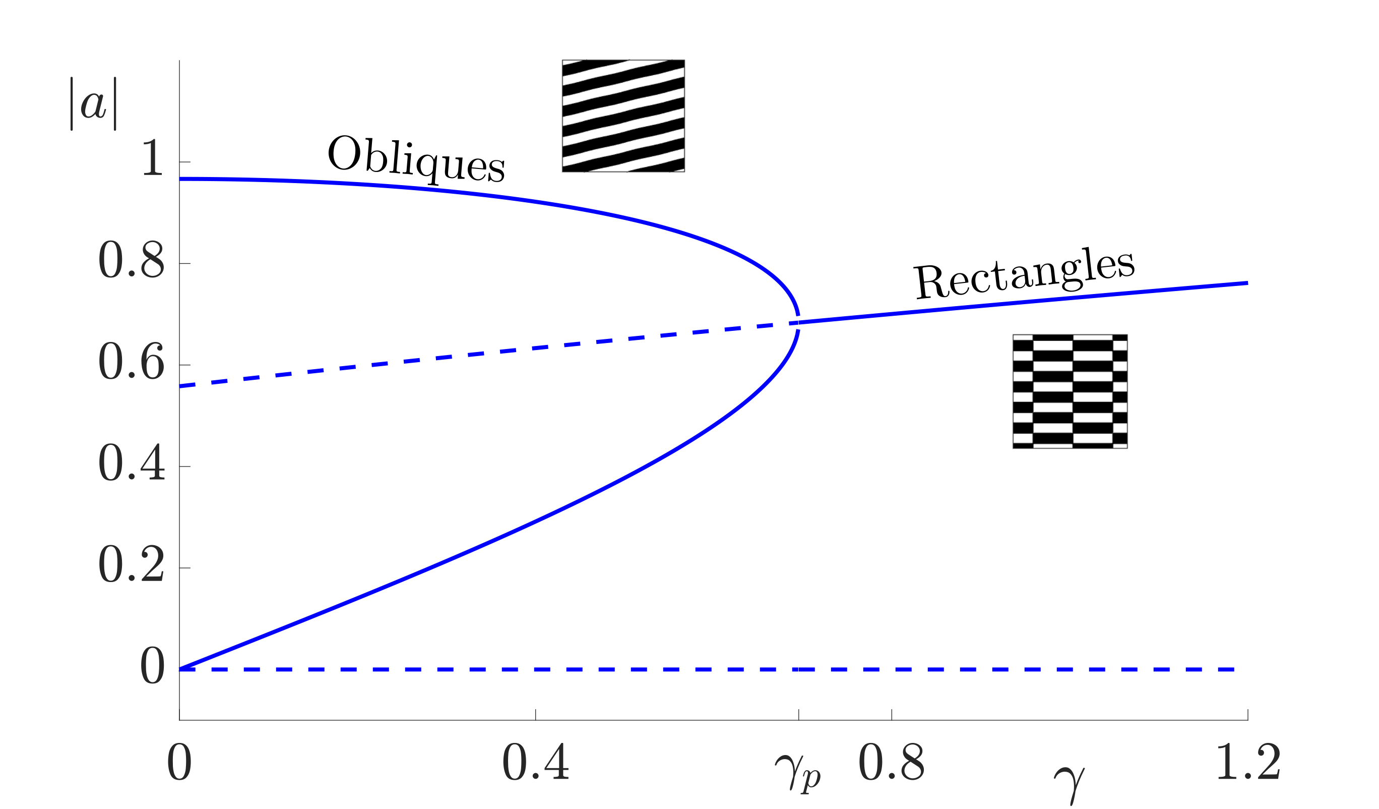
Figure 6: Bifurcation diagram for constant two-dimensional pattern solutions for the forced neural field equation (1). Solid lines indicate stable states while dotted lines indicate unstable solutions. Parameter values are \(\sigma=0.5\), \(h=0\) and \(v_2=0.75 k_0\). Here we hold the distance from Turing instability, \(\epsilon^2\delta= 0.3\), and range over values of \(\gamma\) with the bifurcation between patterned states at \(\gamma_{p} =4\epsilon^2 \delta/ \mu_c\).

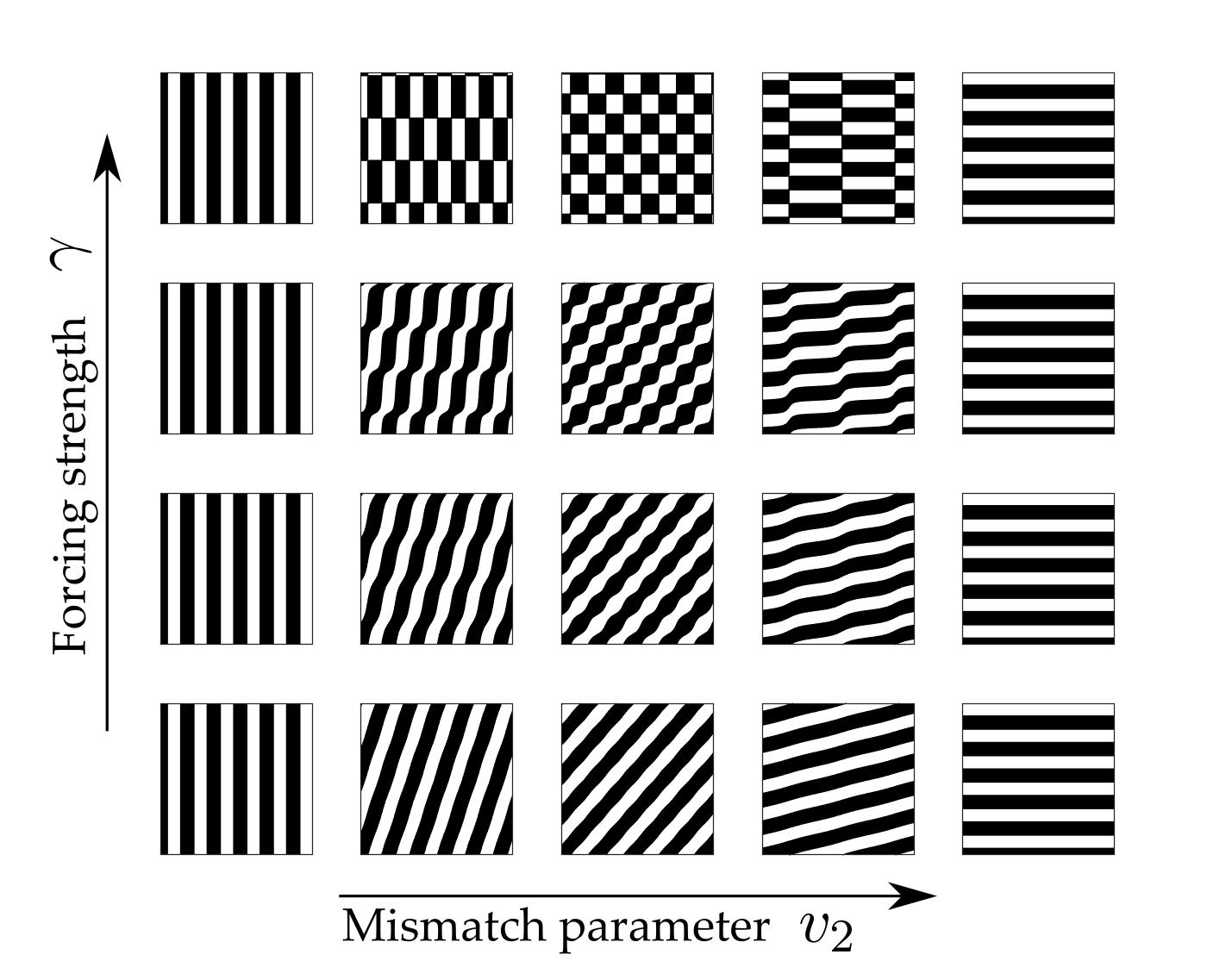
Figure 7: Planforms of the stable leading order solution demonstrating pattern diversity and orthogonal response. As \(v_2\) is increased from \(0\) to \(k_0\) the pattern changes from vertical stripes to rectangles (when \(\gamma> \gamma_p\)) or oblique patterns (when \(\gamma< \gamma_p\)) to horizontal stripes which are orthogonal to the forcing. This corresponds to varying \(k_x\) from \(k_0\) (with a response in the direction of forcing) to \(0\) (with a response orthogonal to the direction of forcing). Other parameter values are \(\sigma=0.5\), \(\epsilon^2 \delta= 0.3\), \(v_2= [ 0, 0.05, 0.25, 0.75, 1]k_0\), \(\gamma=[ 0.1, 0.4, 0.65, 1.1]\). Planforms are plotted for \(x,y\in [0,10\pi]\).

3. Movement through adaptation

Recall that the hallucinations reported by Billock and Tsou [3] included hallucinatory movement in response to retinal stimulation with static patterns. A key requirement for illusory motion is anticipated to be that the neural field model without drive supports travelling and standing wave patterns. We therefore include adaptation (negative feedback) since it provides a description of metabolic processes that lead to fatigue and is also a well known route to dynamic instabilities leading to the formation of travelling waves.

To establish that a neural field model with adaptation and static spatial forcing can support resonant travelling and standing wave patterns, it is sufficient to consider a one-dimensional model (but note that amplitude equations in two-dimensions are developed in [19]). In this case the model for activity \(u(x,t)\) is

\( \frac{\partial}{\partial t}u(x,t) = -u(x, t) + \int_{-\infty}^\infty w(|x- x'|) f(u(x',t); \mu)\, \mbox{d} x' - g\int_{-\infty}^t \eta(t-t')u(x,t') \, \mbox{d} t' + \gamma u(x,t) I(x,t), \)

(8)

where firing rate \(f\) and connectivity kernel \(w\) are as in (2) and (3) respectively and

\( \eta(t) = \frac{1}{\tau_a} \mbox{e}^{-t/\tau_a} H(t), \)

(9)

where \(H\) is a Heaviside step function. The parameter \(g>0\) describes the strength of the adaptive feedback and \(\tau_a>0\) sets the relative timescale.

For the model (8) without drive (\(\gamma=0\)), linear stability analysis of the homogeneous steady state \(u=0\) (which now occurs when we let \(A= \sigma^{-1}\) in (3)) reveals that a dynamic Turing instability to a time dependent patterns with spatial wavenumber \(k_0\) and emergent frequency of oscillation \(\omega_c=\sqrt{\tau_a g -1}/\tau_a\) occurs when \(\widehat{w}(k_0) = (1+\tau_a)/(\tau_a f'(0; \mu_c, h_c))\) for \(\tau_a g>1\) and \(g > f'(0; \mu_c, h_c)\widehat{w}(k_0)-1\). Adding drive of the form \(I(x,t) = \cos(k_f x)\) where \(k_f = 2(k_0-v_1)\) for mismatch parameter \(v_1\) gives rise to solutions of the form

\( u \simeq A(\tau) \mbox{e}^{i(k_x x + \omega_c t)} + B(\tau) \mbox{e}^{i(k_x x - \omega_c t )} + \mbox{ c.c.} \)

(10)

Weakly nonlinear analysis (ignoring slow spatial variation) again gives equations for the dynamics of the amplitudes \(A\) and \(B\) and upon rescaling \(t= \epsilon^{-2} \tau\) the evolution of corresponding amplitudes \(a(t)= \epsilon A(\tau)\), \(b(t)= \epsilon B(\tau)\) is given by the system

\( (1+ g \widetilde{\eta}^\prime(i\omega_c)) \frac{\partial a} {\partial t} = \Lambda a -\widehat{w}(k_0)\left( \Psi_1 |a|^2 + \Psi_2 |b|^2 \right)a + \frac{\gamma}{2} b^* , \)

(11)

\( (1+ g \widetilde{\eta}^\prime(-i\omega_c)) \frac{\partial b} {\partial t} = \Lambda b -\widehat{w}(k_0)\left( \Psi_1^* |b|^2 + \Psi_2^* |a|^2 \right)b + \frac{\gamma}{2} a^* , \)

(12)

where

\( \Psi_1 = -\beta_2\xi(k_0, \omega_c) - 3 \beta_3, \quad \Psi_2 = -2 \beta_2\xi(k_0, 0) - 6\beta_3, \quad \mbox{with} \ \ \xi(k,\omega)= \frac{2 \beta_2 \widehat{w}(2k)}{2\omega i + 1-\beta_c \widehat{w}(2k)+ g\widetilde{\eta}(2\omega i)}, \)

\(\Lambda = \widehat{w}(k_0) \epsilon^2 \delta + \beta_c v_1^2 \widehat{w}^{\prime\prime}(k_0)/2\) and \(\widetilde{\eta} (\lambda) = \int_0^\infty \mbox{d} t \, \eta(t) \mbox{e}^{-\lambda t}\) is the Laplace transform of \(\eta(t)\).

These equations support stable solutions with constant and equal amplitudes, corresponding to periodic (when \(h=0\)) or modulated (when \(h\neq 0\)) standing waves and also solutions with constant unequal amplitudes corresponding to periodic (when \(h=0\)) or amplitude modulated (when \(h\neq 0\)) travelling waves. Numerical investigations suggest that the travelling wave solutions are stable whenever they exist and that there are regions of bistability between modulated standing waves and travelling waves in cases where \(h\neq 0\). The bifurcation diagrams in Fig. 8 indicate that travelling waves are stable for weak forcing and standing waves are stable for larger values of \(\gamma\).

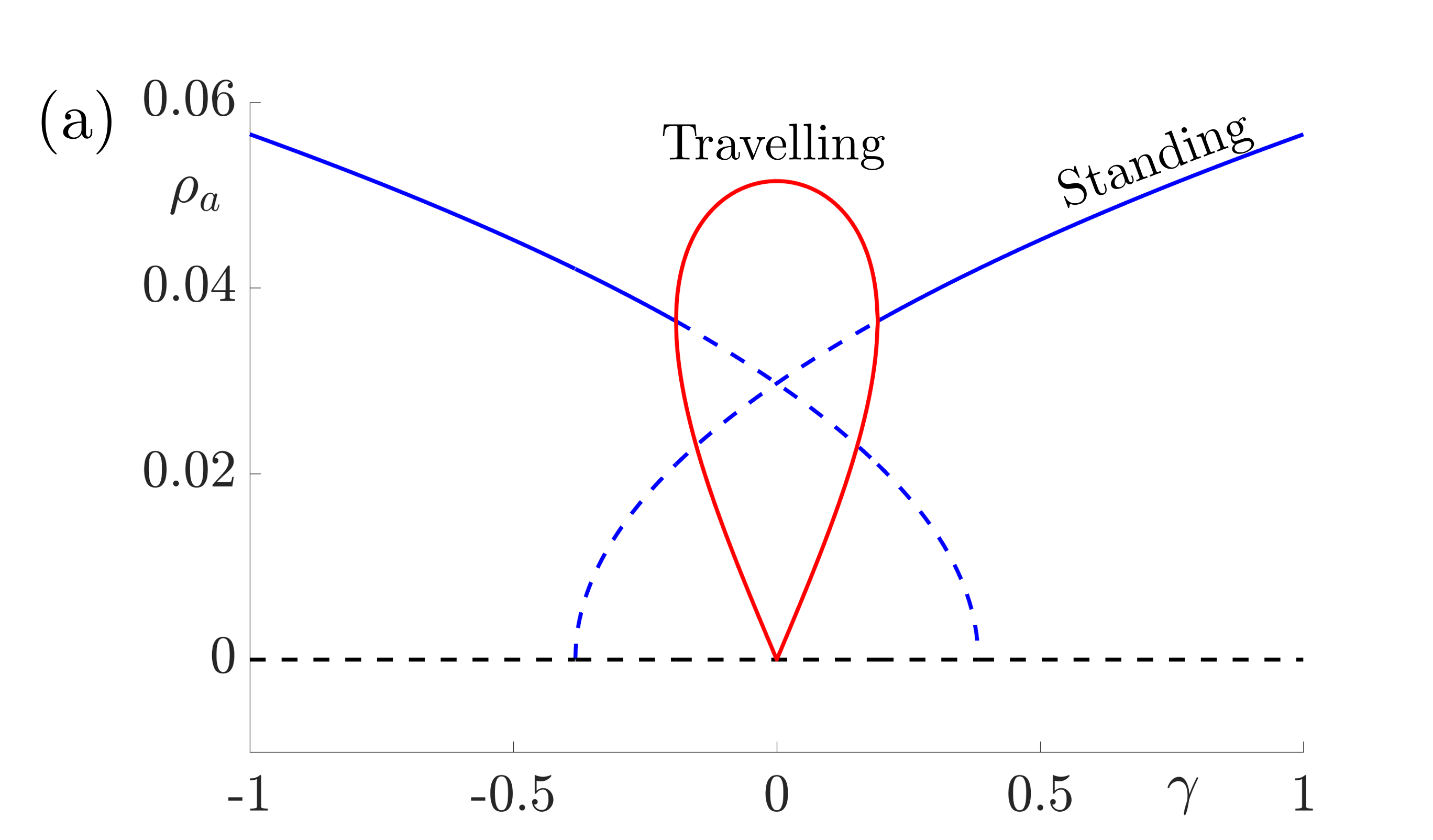
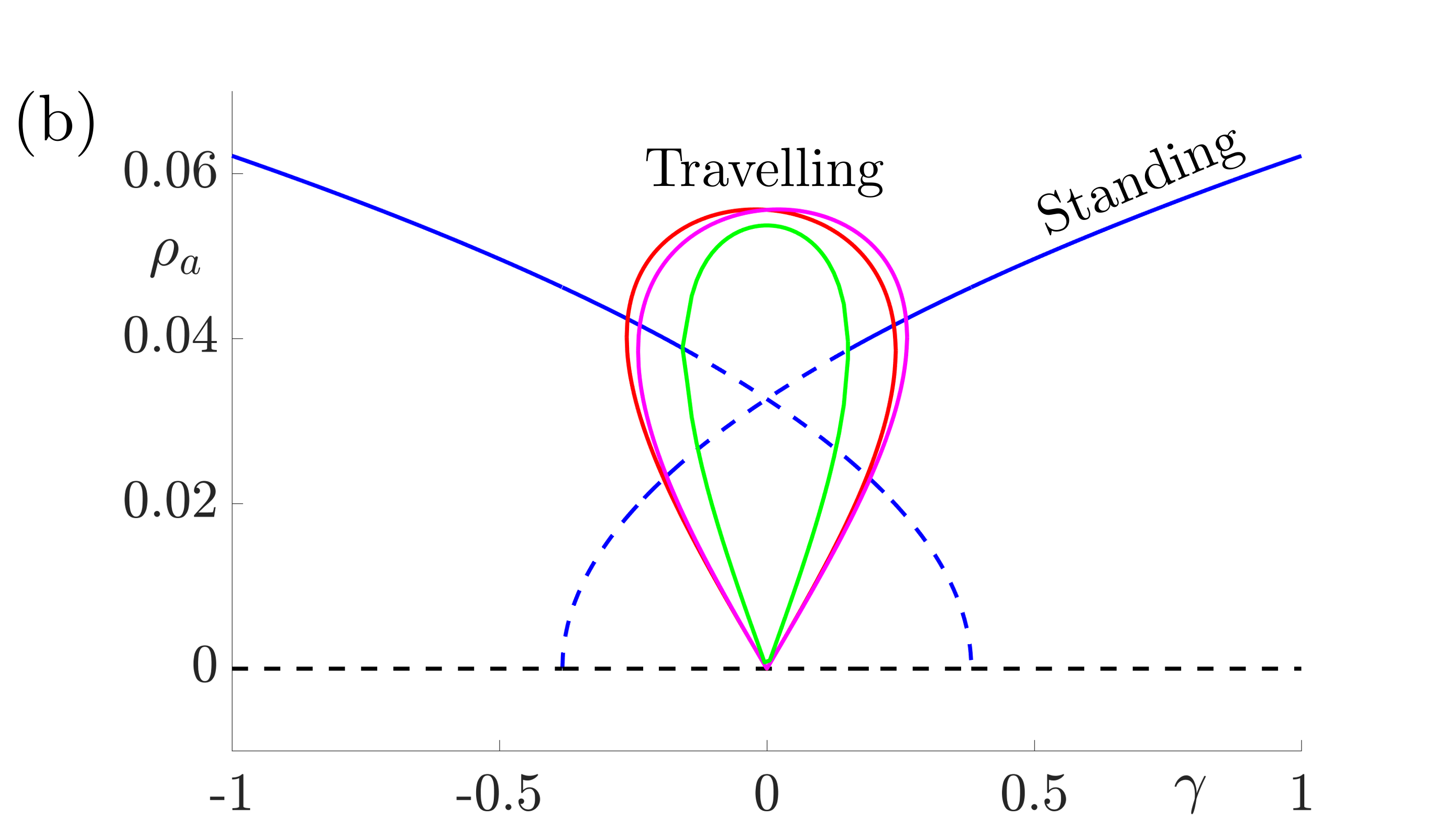
Figure 8: Bifurcation diagrams for resonant stripe pattern solutions in one spatial dimension with adaptation (\(g\neq0\)) under variation of the forcing strength \(\gamma\). In (a) \(h=0\) and we observe periodic standing waves (blue) and travelling waves (red). Dashed lines indicate unstable solutions while solid lines indicate stable waves. In (b) we choose \(|h|=0.05\) and we observe modulated (quasiperiodic) standing (blue) and various travelling (red, magenta and green) waves. Other parameter values for both diagrams are \(\sigma=0.5\), \(\tau_a=1\), \(g=5\). These give \(\beta_c= 3\), \(\widehat{w}(k_0)=2/3\) and \(\widehat{w}^{\prime\prime}(k_0)=-16/27\) and here we take \(\epsilon^2 \delta=0.3\) and \(v_1=0.1\) so that \(\Lambda = \widehat{w}(k_0) \epsilon^2 \delta + \beta_c\widehat{w}^{\prime\prime}(k_0)v_1^2/2= 43/225\).

The conclusion is that when adaptation is included, there are stable \(2\):\(1\) resonant solutions which travel. Investigating the fully two-dimensional model with adaptation numerically reveals the same qualitative behaviour. Moreover, when the unforced system supports traveling waves, resonant rectangular patterns remain stationary but oblique patterns travel in an orthogonal direction, namely along the axis for which the continuous translational symmetry is not broken by the forcing. Thus, if spatial forcing is by a striped pattern along the \(x\)-direction then the tissue response could be a striped pattern in the orthogonal \(y\)-direction. Moreover, the presence of adaptation would allow for a dynamic instability so that this could propagate as a plane wave.

4. Simulations and psychophysics

We now turn to the perception of patterns of activity in V1. The log-polar mapping [24] is perhaps the most common representation of the mapping of points from the retina to the visual cortex and see Fig. 3. Thus to answer how an activity pattern would be perceived we need only apply the inverse (conformal) log-polar mapping. The analytical work summarised in the previous sections has established that an orthogonal response to global spatially periodic forcing can be robustly supported in a standard neural field model. Therefore, if the conditions for a resonant response are met, then a visual stimulus in the form of a set of concentric rings may give rise to a percept of a set of radial arms. Similarly, a visual stimulus in the form of a set of radial arms may give rise to a percept of a set of concentric rings. This is consistent with the observations of Billock and Tsou as described in the introduction, albeit these are more accurately described by drive on the cortical half-space (since the stimuli do not cover the whole visual field). However, direct numerical simulations including forcing with striped patterns on the cortical half-space are seen to recover all of the features reported in Fig. 3, once the inverse retino-cortical map is applied. The corresponding plots for cortical activity are shown in Fig. 9. The presence of the adaptation current allows the formation of travelling striped patterns, and these correspond to rotating waves in the retinal space with blinking versions associated to standing waves. Although the psychophysical experiments of Billock and Tsou involve a component of temporal flicker we have found that it is not strictly necessary to include this within the model to generate results consistent with their observations. Nonetheless, direct numerical simulations with flicker do show that the phenomenon is robust to this inclusion. We posit that in the psychophysical experiments the background flicker helps put the primary visual cortex in a state conducive to a \(2\):\(1\) resonance, whereas here the intrinsic parameters are tuned to reach this condition.

Figure 9: Simulation results from a neural field model with spatially periodic striped forcing on the half-space. (a) Horizontal stripes forcing the left half-space give rise to stationary vertical stripes on the right. (b) Vertical stripes forcing the left half-space give rise to travelling horizontal stripes on the right. (c) Horizontal stripes forcing the right half-space give rise to stationary vertical stripes on the left. (d) Vertical stripes forcing the right half-space give rise to travelling horizontal stripes on the left. An application of the inverse retino-cortical map to (a), \(\ldots\), (d) generates patterns consistent with (a), \(\ldots\), (d) shown in Fig. 3. Parameter values are \(\sigma=0.8\), \(\mu=2\), \(h=0.05\), \(\gamma=0.5\) and for b) and d) \(\tau_a = 10\), \(g = 0.14\). The domain sizes are a) \([-16.53,16.53] \times [-15.71,15.71]\), b) \([-31.42,31.42] \times [-3.10,3.10]\), c) \([-22.73,22.73] \times [-22.00,22.00]\) and d) \([-31.42,31.42] \times [-2.07,2.07]\) with periodic boundary conditions. Click on the four animations above to see the full size videos.

5. Future directions

Here we have focused on the analysis of simple spatially repetitive and time-independent stimuli. Even simple variants of such patterns, such as the Enigma, created by pop-artist Isia Leviant [12], consisting of concentric annuli on top of a pattern of radial spokes, can lead to very striking illusory motion percepts. An extension of the work described in this article would be to consider input patterns with more spatial structure and explore the conditions for the emergence of global illusory percepts from local interactions, such as the Barberpole, Café wall, Fraser spiral, and Ehrenstein illusion in which local orientation differences lead to the appearance of the global rotation of contours (see [10] for further examples). Moreover, given that periodic and quasi-crystal patterns in physical (Faraday) systems can be excited by periodic temporal forcing [21] this motivates a further study of associated behaviour in neural models. It is known that full-field flickering visual stimulation in humans can produce geometric hallucinations in the form of radial or spiral arms (and conversely that brain rhythms at the flicker frequency can be enhanced with the presentation of static radial or spiral arms) [18]. Indeed, flicker induced hallucinations have previously been studied from a theoretical perspective in neural fields with time periodic forcing by Rule et al. [22], and it would be very natural to extend the work here to include models of spatio-temporal sensory drive, and in particular to further understand visual hallucinations induced by flicker constrained to a thin annulus centred on the fovea [20]. Another natural extension is to extend very recent work on undriven neural fields that shows how quasi-crystal patterns can arise via a Turing instability [9] to further include spatio-temporal forcing.

Acknowledgement

The author would like to thank Stephen Coombes for his helpful comments on drafts of this article.

References

[1]   S. Amari, Dynamics of pattern formation in lateral-inhibition type neural fields, Biological Cybernetics, 27 (1977), pp. 77-87.

[2]   M. Balasubramanian, J. Polimeni, and E. L. Schwartz, The V1-V2-V3 complex: Quasiconformal dipole maps in primate striate and extra-striate cortex, Neural Networks, 15 (2002), pp. 1157-1163.

[3]   V. A. Billock and B. H. Tsou, Neural interactions between flicker-induced self-organized visual hallucinations and physical stimuli, Proceedings of the National Academy of Sciences, 104 (2007), pp. 8490-8495.

[4]   P. C. Bressloff, J. D. Cowan, M. Golubitsky, P. J. Thomas, and M. Wiener, Geometric visual hallucinations, {E}uclidean symmetry and the functional architecture of striate cortex, Philosophical Transactions of the Royal Society London B, 40 (2001), pp. 299-330.

[5]   B. R. Conway, A. Kitaoka, A. Yazdanbakhsh, C. C. Pack, and M. S. Livingstone, Neural basis for a powerful static motion illusion, Journal of Neuroscience, 25 (2005), pp. 5651-5656.

[6]   S. Coombes, P. beim Graben, R. Potthast, and J. Wright, eds., Neural Fields: Theory and Applications, Springer, 2014.

[7]   G. B. Ermentrout, Neural networks as spatio-temporal pattern-forming systems, Reports on Progress in Physics, 61 (1998), pp. 353-430.

[8]   G. B. Ermentrout and J. D. Cowan, A mathematical theory of visual hallucination patterns, Biological Cybernetics, 34 (1979), pp. 137-150.

[9]   A. Gökçe, D. Avitabile, and S. Coombes, Quasicrystal patterns in a neural field model, Physical Review Research, 2 (2020), p. 013234.

[10]   A. Kitaoka, Akiyoshi's illusion pages, http://www.ritsumei.ac.jp/~akitaoka/index-e.html.

[11]   H. Kluver, Mescal and Mechanisms of Hallucinations, University of Chicago Press, Chicago, 1966.

[12]   I. Léviant, Illusory Motion within Still Pictures: The L-Effect, Leonardo, 15 (1982), pp. 222-223.

[13]   D. M. Mackay, Moving visual images produced by regular stationary patterns, Nature, 180 (1957), pp. 849-850.

[14]   R. Manor, A. Hagberg, and E. Meron, Wave-number locking in spatially forced pattern-forming systems, {EPL} (Europhysics Letters), 83 (2008), p. 10005.

[15]   R. Manor, A. Hagberg, and E. Meron, Wavenumber locking and pattern formation in spatially forced systems, New Journal of Physics, 11 (2009), p. 63016.

[16]   Y. Mau, A. Hagberg, and E. Meron, Spatial Periodic Forcing Can Displace Patterns It Is Intended to Control, Physical Review Letters, 034102 (2012), pp. 1-5.

[17]   Y. Mau, L. Haim, A. Hagberg, and E. Meron, Competing resonances in spatially forced pattern-forming systems, Physical Review E, 88 (2013), pp. 1-9.

[18]   F. Mauro, A. Raffone, and R. VanRullen, A bidirectional link between brain oscillations and geometric patterns, Journal of Neuroscience, 35 (2015), pp. 7921-7926.

[19]   R. Nicks, A. Cocks, D. Avitabile, A. Johnston, and S. Coombes, Understanding sensory induced hallucinations: From neural fields to amplitude equations, SIAM Journal on Applied Dynamical Systems, 20 (2021), pp. 1683–1714.

[20]   J. Pearson, R. Chiou, S. Rogers, M. Wicken, S. Heitmann, and B. Ermentrout, Sensory dynamics of visual hallucinations in the normal population, eLife, 5 (2016), p. e17072.

[21]   A. M. Rucklidge and M. Silber, Quasipatterns in parametrically forced systems, Physical Review E, 75 (2007), p. 055203.

[22]   M. Rule, M. Stoffregen, and B. Ermentrout, A model for the origin and properties of flicker-induced geometric phosphenes, PLOS Computational Biology, 7 (2011), pp. 1-14.

[23]   E. Schwartz, Spatial mapping in the primate sensory projection: analytic structure and relevance to projection, Biological Cybernetics, 25 (1977), pp. 181-194.

[24]   E. L. Schwartz, Computational anatomy and functional architecture of striate cortex: A spatial mapping approach to perceptual coding, Vision Research, 20 (1980), pp. 645-669.

[25]   R. Sokoliuk and R. VanRullen, The flickering wheel illusion: when \(\alpha\) rhythms make a static wheel flicker, Journal of Neuroscience, 33 (2013), pp. 13498-13504.

[26]   C. W. Tyler, Traversing the highwire from pop to optical, PLoS Biology, 3 (2005), p. e136.