Jonathan Jaquette, Department of Mathematics and Statistics, Boston University, Boston, MA 02215, USA ([email protected]).

Author's Note: The figures used in this article are reproduced with permission from [BJ21].

1. Introduction

Coherent structures, such as standing waves and traveling pulses, are emblematic examples of the dynamics in nonlinear PDEs. Beyond the question of existence, understanding a structure's stability is of central interest. Whereas an unstable wave repels nearby trajectories, a stable wave will be robust under perturbation and could be expected to be experimentally observable. In parabolic PDEs with a single spatial dimension, one can make a traveling wave ansatz essentially reducing the problem to an ODE. However computing stability of waves, especially in large systems of PDEs, is still difficult.

A standard tool for computing stability is the Evans function \(E(\lambda)\), an complex analytic function whose zeros correspond to eigenvalues in the point spectrum. By using Cauchy's argument principal, one can count the number of eigenvalues inside a contour \(\Gamma \subseteq \mathbb{C}\) by computing the winding number of the image \(E(\Gamma)\).

In recent years there has been considerable scholarship developing a new approach to computing stability [BCC+20, BCJ+18, JLS16, CJ20, CJM15, DJ11, How20, HLS18, JLM13]. This method uses the Maslov index to equate the number of unstable eigenvalues with the number of so-called conjugate points, and has been surveyed in the Notices of the AMS [Bec20] and a recent SIAM DS-Web Magazine article [Cor21].

In this article we describe how these conjugate point techniques can be applied to numerically compute stability of standing waves in a particular class of PDEs. These methods are efficient, roughly equivalent to evaluating the Evans function at just a single value of \(\lambda=0\). Moreover, by employing validated numerics we are able to give computer assisted proofs of stability in concrete examples [BJ21].

1.1. Reaction Diffusion Systems with a Gradient Nonlinearity

Consider a reaction diffusion equation with a gradient nonlinearity

\( u_t = D u_{xx} + \nabla G(u) , \qquad u \in \mathbb{R}^{n} \qquad x \in \mathbb{R} \)

(1)

for diffusion matrix \(D\) and nonlinearity \(G \in C^{2}(\mathbb{R}^{n} , \mathbb{R}^{n})\). For a stationary solution \(\varphi(x) : \mathbb{R}\to \mathbb{R}^{n}\) one obtains the eigenvalue problem

\( \lambda u = { D u_{xx} + \mathcal{M}(x) u =: \mathcal{L} u}, \qquad u \in \mathbb{R}^{n} , \qquad x \in \mathbb{R} \)

(2)

where \(\mathcal{M}(x) = \nabla^2G(\varphi(x))\) is symmetric. The spectrum of \(\mathcal{L}\) can be divided into two disjoint sets: the essential spectrum, which is relatively easy to compute, and the point spectrum, which is not.

For our analysis, we begin by rewriting our eigenvalue equation (2) as a first order system, taking \( U = ( u , D u_x) \in \mathbb{R}^{2n}\) and obtaining

\( U_x = J \mathcal{B}(x;\lambda) U , \mathcal{B} (x;\lambda) = \begin{pmatrix} \lambda - \mathcal{M}(x) \qquad\quad 0 \\ 0 \qquad\qquad - D^{-1} \end{pmatrix}, \)

(3)

where \(J = \left(\begin{smallmatrix} 0 & - Id \\ Id&  0 \end{smallmatrix} \right)\) is a symplectic matrix. A value \(\lambda \in \mathbb{R}\) and solution \(U:\mathbb{R}\to \mathbb{R}^{2n}\) to (3) is an eigenpair if and only if

\( \lim_{x \to \pm \infty} |U(x)| = 0 \)

To focus on solutions which go to \(0\) as \(x \to \pm \infty\) one defines the (un)stable subspaces:

\( \mathbb{E}^{u}_{-}(x;\lambda) := \{ U(x) : U(x)\) solves (3) and \(U(x) \to 0\) as \(x \to - \infty \}\) \(\mathbb{E}^{s}_{+}(x;\lambda) := \{ U(x) : U(x)\) solves (3) and \(U(x) \to 0\) as \(x \to + \infty \}. \)

As (3) is a linear non-autonomous ODE, then \(\mathbb{E}^{u}_{-}(x;\lambda) \subset \mathbb{R}^{2n}\) and \(\mathbb{E}^{s}_{+}(x;\lambda) \subset \mathbb{R}^{2n}\) are linear subspaces for all \(x\) and \(\lambda\). In this notation \(\lambda\) is an eigenvalue if and only if \(\mathbb{E}^{u}_{-}(x;\lambda) \cap \mathbb{E}^{s}_{+}(x;\lambda) \neq \{ 0\}\).

To further characterize the asymptotic behavior of the system (3) at \(x = \pm \infty\), we define the matrices \(J \mathcal{B}_{\pm}(\lambda) := \lim_{x \to \pm \infty} J \mathcal{B}(x; \lambda )\). Thereby as \(x \to \pm \infty\), the subspaces \(\mathbb{E}^{u/s}_{\pm}(x;\lambda)\) limit to the (un)stable eigenspaces of \(J \mathcal{B}_{\pm}(\lambda)\). We will also make the mild assumption that \(J \mathcal{B}_{\pm}(0)\) is hyperbolic with \(n\) positive and \(n\) negative eigenvalues, whereby each of \(\mathbb{E}^{u/s}_{\pm}(x;0)\) is an \(n\) dimensional subspace.

2. Connecting the stability of waves with topology

For the classical Sturm-Liouville eigenvalue problem (compare with (2) on a bounded domain with \(n=1\)) there may only exist real eigenvalues \(\lambda_0 > \lambda_1 > \lambda_2 \dots\). Moreover, the eigenfunction associated with \(\lambda_m\) has precisely \(m\) zeros. Note that If \(\varphi\) is a stationary solution to (1) then its derivative automatically solves the linearized equation (3) with eigenvalue \(\lambda=0\). If \(0=\lambda_m\) is the \(m\)th eigenvalue, then it's eigenfunction \(\varphi'(x)\) must possess \(m\) zeros. Conversely, by counting the number of zeros of \(\varphi'(x)\), one is able to determine the number of positive eigenvalues in the point spectrum of \(\mathcal{L}\). As a result, any scalar pulse is necessarily unstable, and any monotonic standing wave is stable.

One would like a way to generalize this approach to systems of equations. By virtue of the derivative of \(\varphi\) being a \(0\)-eigenvalue, we have for any \(n\in \mathbb{N}\) that

\( \begin{pmatrix} \varphi'(x) \\ D\varphi''(x) \end{pmatrix} \in \mathbb{E}^u_-(x;0) \cap \mathbb{E}^s_+(x;0). \)

In the scalar case the derivative \(\varphi\) spans the entire space \(n=1\) dimensional space \(\mathbb{E}^u_-(x;0)\), however this is not true for \(n\geq 2\). The key to generalizing these type of Sturm Liouville results is through studying \(\mathbb{E}^u_-(x;0)\), and in particular exploiting the symplectic structure in (3).

To describe how symplectic geometry factors into the equation, let us define a symplectic form by

\( \omega : \mathbb{R}^{2n} \times \mathbb{R}^{2n} \to \mathbb{R} \qquad \omega( U,W) = \left\langle U, J W \right\rangle \)

for the standard inner product \(\left\langle \cdot , \cdot \right\rangle\) and vectors \(U,W \in \mathbb{R}^{2n}\). Since the matrix \(\mathcal{B}(x;\lambda)\) is symmetric, one can show that the symplectic form is preserved under the flow; that is if \(U(x)\) and \(W(x)\) both solve (3) then \(\frac{d}{dx} \omega ( U(x),W(x)) = 0\). It turns out that each subspace \(\mathbb{E}^u_-(x;\lambda)\) is Lagrangian, which is to say that \(\omega (U,W) = 0\) for all \(U,W \in \mathbb{E}^u_-(x;\lambda)\). Hence, we may think of \(\mathbb{E}^u_-(x;\lambda)\) as tracing out a path in the Lagrangian Grassmanian:

\( \Lambda(n) := \left\{ \ell \subset \mathbb{R}^{2n} : \dim ( \ell ) = n , \;\; \omega ( U,W) = 0 \;\; \forall U,W \in \ell \right\}. \)

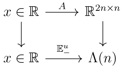
It turns out that \(\Lambda(n)\) may be identified with the quotient \(\Lambda(n) \cong U(n) / O(n)\), see Figure 1. Furthermore the determinant squared map \({\det}^2 : U(n) / O(n) \to \mathbb{S}^1 \subseteq \mathbb{C}\) induces an isomorphism of fundamental groups. Thus \(\pi_1(\Lambda(n)) = \mathbb{Z}\) and Maslov index measures the homotopy type of paths in \(\Lambda(n)\). As we will see, the Maslov index is the key to computing stability.

Figure 1: Cartoon picture of \(\Lambda(2)\), which is double covered by \(\mathbb{S}^1 \times \mathbb{S}^2\). The blue squares are identified under the quotient and represent \(\mathcal{D}\); the blue circles represent \(\mathcal{T}\); the green path represents \(\mathbb{E}_-^u(x;0)\); the solid red square represents the unstable eigenspace of \(J\mathcal{B}_{-}(0)\).

For a loop in the plane \(\gamma : \mathbb{S}^1 \to \mathbb{R}^2\) there are several ways to compute its winding number about a point \(x_0 \in \mathbb{R}^2\). One such method is to fix a horizontal ray emanating from \(x_0\), and then count the number of time \(\gamma\) crosses the ray going up, minus the number of times \(\gamma\) crosses the ray going down. This is analogous to a track coach counting the number of laps a runner completes by counting the number of times, and direction through which, they cross the starting line.

In a similar fashion we may compute the Maslov index by fixing a reference plane, and counting the number of times the path \(\mathbb{E}_-^u(x;0)\) crosses through it. To that end, we define the Dirichlet subspace as

\( \mathcal{D} = \big\{ (u,v) \in \mathbb{R}^{2n } : u = 0 \big\}, \)

and define the train of \(\mathcal{D}\) as the set of Lagrangian planes which intersect \( \mathcal{D}\)

\( \mathcal{T} = \big\{ \ell \in \Lambda(n) : \ell \cap \mathcal{D} \neq \{0\} \big\}. \)

Definition 2.1. For fixed \(\lambda = 0\), define conjugate points as values of \(x\) such that \(\mathbb{E}_-^u(x;0) \in \mathcal{T}\).

For the PDE in (1) it turns out that \(\mathbb{E}_-^u(x;0)\) always passes through \(\mathcal{T}\) in the same direction. Moreover, in [BCJ+18] it is shown that conjugate points are in correspondence with unstable eigenvalues.

Theorem 2.2. The number of positive eigenvalues of \(\mathcal{L}\) is equal to the number of conjugate points. All conjugate points are in \([ -L_- , L_+]\) for some \(L_-, L_+ \in \mathbb{R}\).

From this, Beck et al. are able to show that symmetric pulses to (1) are necessarily unstable. To see this, note that if \(\varphi(x) = \varphi(-x)\) is a pulse, then \(\varphi'(0)=\vec{0}\). As \((\varphi'(x),D\varphi''(x)) \in \mathbb{E}_-^u(x;0)\) is an eigenfunction and \((\varphi'(0),D\varphi''(0)) \in \mathcal{D}\), then it follows that \(0\) is a conjugate point. Hence there exists at least one positive eigenvalue. This result nicely complements the Sturm-Liouville theory, wherein pulse solutions to scalar PDEs are necessarily unstable. Contrastingly, as we will see in Section 4, there exist both stable and unstable standing waves in the PDE (1).

3. Computing Conjugate Points in Practice

So how does one go about computing conjugate points? In order to determine whether \(\mathbb{E}_-^u(x;0) \in \mathcal{T}\), it is helpful to work with a representative for \(\mathbb{E}_-^u(x;0)\). We say that \(A(x) = \begin{pmatrix} A_1(x) \\ A_2(x) \end{pmatrix}\) is a frame matrix for \(\mathbb{E}_-^u(x)\) if its columns span \(\mathbb{E}_-^u(x;0)\). Clearly a choice of frame matrix is not unique. But note that \(\mathbb{E}_-^u(x;0) \in \mathcal{T}\) if and only if there exists a linear combination of the columns of \(A_1(x)\) which produces the \(0\)-vector. Moreover we have the following lemma:

Lemma 3.1. The value \(x\in \mathbb{R}\) is a conjugate point if and only if \(\det A_1(x) = 0\).

The overall approach to computing conjugate points may be summarized as follows:

• Compute a stationary solution to (1).
• Compute a frame matrix \(A(x)\) for \(\mathbb{E}_-^u(x;0)\).
• Identify constants \(L_-,L_+ \geq 0\) such that all conjugate points are in \([-L_- , L_+]\).
• Enumerate all the zeros of \(\det A_1(x)\) in the interval \([-L_-,L_+]\).

To begin, first one must compute a stationary solution \(\varphi(x) : \mathbb{R}\to \mathbb{R}^{n}\) to the PDE (1). Such a solution corresponds to a connecting orbit \(\phi = ( \varphi, D \varphi_x)\) to the Hamiltonian ODE

\( H(v,w) = \tfrac{1}{2} \| D^{-1} w\|^2 + G(v) \\ (v,w)' = - J \nabla H(v,w). \)

If there exists a heteroclinic solution between equilibria \(p_0\) and \(p_1\), then it is necessary that \(H(p_0) = H(p_1)\). In this context, one can solve for a connecting orbit as a boundary value problem between the unstable manifold of \(p_0\) and the stable manifold of \(p_1\), see Figure 2. In some special cases one might have an analytic solution for a connecting orbit, but often they are only explicitly accessible by numerics. A considerable amount of scholarship has been dedicated to computation of connecting orbits, more than we could hope to fully survey. For references using validated numerics / computer assisted proofs we direct the reader to [Ois98, WZ03, vdBDLMJ15, AK15, CZ17, vdBBLM18, vdBS20] and the references cited therein.

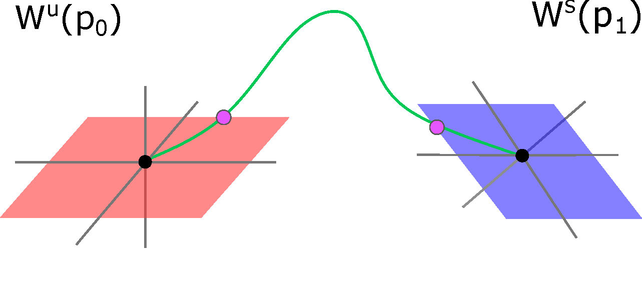
Figure 2: A cartoon of a heteroclinic orbit.

To compute a frame matrix, recall that as \(x \to - \infty\) then \(\mathbb{E}^{u}_{-}(x;0)\) limits to the unstable eigenspace of \(J \mathcal{B}_-\). Let \(v_k\) be the unstable eigenvectors of \(JB_-\), and define \(\mathcal{V}^u_- = [ v_1 | \dots |v_n]\). Thereby, \(\mathbb{E}^u_-(x;0)\) has a frame matrix

\( A(x) = \mathcal{V}^u_- + E(x) \)

where \(E(x) \to 0\) as \(x \to - \infty\). Using exponential dichotomies we are able to obtain explicit control on the size of \(\|E(x)\|\). Moreover, one may prove that if \(L_-\) is sufficiently large (and with explicitly verifiable conditions), then there do not exist any conjugate points \(x \in (-\infty, -L_-]\).

Our next goal is to extend our frame matrix \(A(x)\) to be defined for \(x \in [-L_-,L_+]\) for some \(L_+ \geq 0\). As \(\mathbb{E}_-^u(x;0)\) was defined to be a subspace of solutions, then one may obtain a frame matrix \(A(x) = [ a_1(x) | \dots | a_n(x)]\) by solving each column \(a_k(x)\) according to the initial value problem in (3). In practice, we only know the initial frame matrix \(A(-L_-) = \mathcal{V}^u_- + E(-L_-)\) with a certain bound on the error \(\|E(-L_-)\|\). By using validated numerical integration we are able to propagate these error bounds forward, and obtain a validated enclosure of the frame matrix. Moreover, one may prove that if \(L_+\) is sufficiently large (and with explicitly verifiable conditions), then there do not exist any conjugate points \(x \in [L_+, +\infty)\).

In this manner, we are able to identify a finite interval \([-L_- , L_+]\) which contains all of the conjugate points, should they exist. To enumerate all of the conjugate points we use Lemma 3.1, which reduces the problem to finding all points \(x \in [-L_-,L_+]\) such that \(\det A_1(x)=0\). As we have explicit control on \(\det A_1(x)\) and its derivative, we are able to obtain a rigorous count the number of zeros on \([-L_-,L_+]\).

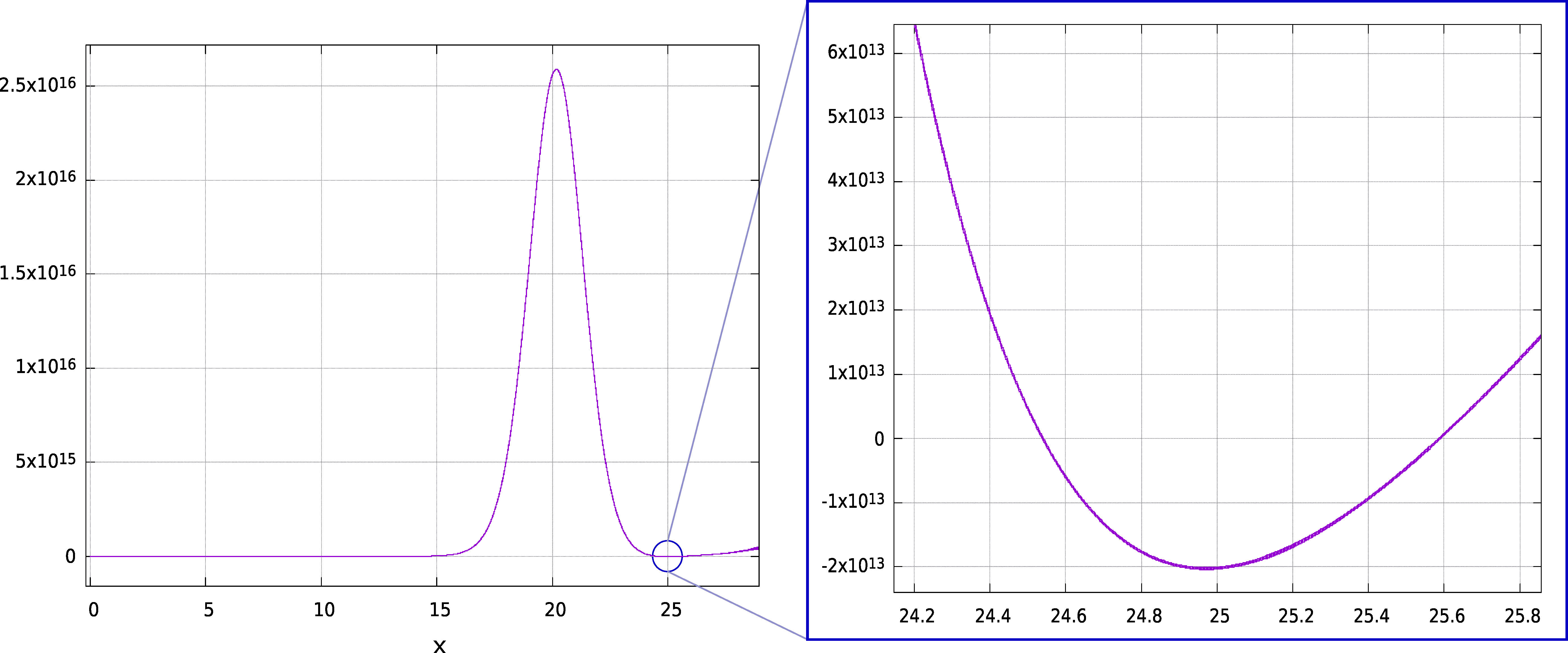
Figure 3: Graph of \(\det A_1(x)\) with two conjugate point for the wave \(\varphi_{++}\) in Theorem 4.1.

4. Applications: Coupled Bistable Equations

For a specific example, let us consider the PDE in (1) with \(D = Id\) and the function \(G\) defined as

\( G(u_1,\dots,u_n) = - \underbrace{ \tfrac{1}{4} \sum_{1 \leq i \leq n } b_iu_i^2 (1-u_i)^2 }_{\mbox{bistable equation}} -\underbrace{ \tfrac{1}{2} \sum_{1 \leq i \leq n-1} c_{i, i+1} u_i (1 - u_i ) u_{i+1} ( 1 - u_{i+1})}_{\mbox{coupling terms}}. \)

with parameters \(b \in \mathbb{R}^n\), \(c = \{ c_{i,i+1}\}_{i=1}^{n-1} \in \mathbb{R}^{n-1}\). For \(n=1\) this is simply the bistable equation,

\( \partial_t u = \partial_x^2 u + b \, f(u) \)

(4)

where \(f(u) = u( u - \tfrac{1}{2})(1-u)\). This PDE has an explicit standing front \(\phi_0(x;b) := \left(1 + e^{-x \sqrt{b/2} } \right)^{-1}\), see Figure 4. The derivative of this standing wave is never zero, so by Sturm-Liouville theory this standing wave is spectrally stable.

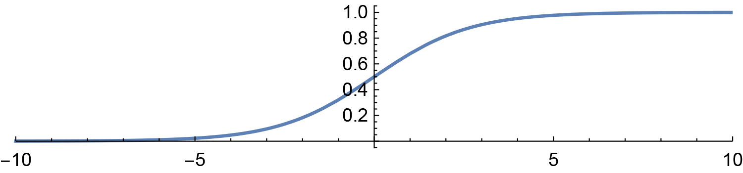
Figure 4: A standing wave to equation (4).

For \(n=3\), the PDE becomes

\( \partial_t u_1 { = \partial_x^2 u_1 + b_1 f(u_1) } + c_{12} g(u_1,u_2) \\ \partial_t u_2 { = \partial_x^2 u_2 + b_2 f(u_2) } + c_{12} g(u_2,u_1) + c_{23} g(u_2,u_3) \\ \partial_t u_3 { = \partial_x^2 u_3 + b_3 f(u_3) } + c_{23} g(u_3,u_2), \)

(5)

where \(g(u, w) = w(1-w)(u- \tfrac{1}{2})\). For the uncoupled case \(c = 0\) this PDE (5) has an explicit front

\( \Phi_0(x) = \left( \phi_0(x;b_1) , \phi_0(x;b_2) , \phi_0(x;b_3) \right). \)

When \(c=0\) this explicit front has a zero eigenvalue with multiplicity three, essentially corresponding to one's ability to translate each of the components independently. For nonzero values of \(c\), we may use the methodology described in section 3 to compute standing waves and their stability. Moreover, in [BJ21] we obtain a computer-assisted-proof of the following theorem:

Theorem 4.1. Fix the parameter \(b = (b_1,b_2,b_3)=(1,.98,.96)\). At each of the four parameter combinations

\( c_{\pm,\pm} = (\pm c_{12}, \pm c_{23}) = ( \pm .04, \pm .02) \)

there exists a standing wave solution \(\varphi_{\pm,\pm}\) to (5) such that

\( \lim_{x \to - \infty} \varphi_{\pm,\pm} (x) = (0,0,0), \qquad \lim_{x \to +\infty} \varphi_{\pm,\pm} (x) = (1,1,1). \)

Furthermore, there are exactly

• \(0\) positive eigenvalues in the point spectrum of \(\varphi_{-,-}\).
• \(1\) positive eigenvalue in the point spectrum of both \(\varphi_{+,-}\) and \(\varphi_{-,+}\).
• \(2\) positive eigenvalues in the point spectrum of \(\varphi_{+,+}\).

In conclusion, through studying the topological properties of \(\mathbb{E}_-^u(x;0)\), computing conjugate points offers an elegant method for determining the stability of coherent structures in PDEs. This method is computationally efficient as well. Whereas with the Evans function approach, one needs to compute \(\mathbb{E}_-^u(x;\lambda)\) for an entire contour of \(\lambda \in \mathbb{C}\), the conjugate point approach only requires one to compute \(\mathbb{E}_-^u(x;0)\) for a single \(\lambda =0\). That said, the conjugate point approach is heavily dependent on the symplectic structure in the problem. Nevertheless, recent work has been extending these techniques to cases where there isn't a nature symplectic structure and beyond [BCC+20].

References

[AK15]   G. Arioli and H. Koch, Existence and stability of traveling pulse solutions of the FitzHugh-Nagumo equation, Nonlinear Anal., 113 (2015), pp. 51-70, https://doi.org/10.1016/j.na.2014.09.023.

[BCC+20]   T. J. Baird, P. Cornwell, G. Cox, C. Jones, and R. Marangell, A Maslov index for non-Hamiltonian systems, arXiv preprint arXiv:2006.14517, 2020.

[BCJ+18]   M. Beck, G. Cox, C. Jones, Y. Latushkin, K. McQuighan, and A. Sukhtayev, Instability of pulses in gradient reaction-diffusion systems: a symplectic approach, Philos. Trans. Roy. Soc. A, 376, 20 (2018), pp. 20170187.

[Bec20]   M. Beck, Spectral stability and spatial dynamics in partial differential equations, Notices of the American Mathematical Society, 67 (2020), pp. 500-507.

[BJ21]   M. Beck and J. Jaquette, Validated spectral stability via conjugate points, arXiv preprint arXiv:2105.06895, 2021.

[CJ20]   P. Cornwall and C. Jones, Bifurcation to instability through the lens of the Maslov index, Preprint, 2020.

[CJLS16]   G. Cox, C. K. R. T. Jones, Y. Latushkin, and A. Sukhtayev, The Morse and Maslov indices for multidimensional Schrödinger operators with matrix-valued potentials, Trans. Amer. Math. Soc., 368 (2016), pp. 8145-8207, https://doi.org/10.1090/tran/6801.

[CJM15]   G. Cox, C. K. R. T. Jones, and J. L. Marzuola, A Morse index theorem for elliptic operators on bounded domains, Comm. Partial Differential Equations, 40 (2015), pp. 1467-1497, https://doi.org/10.1080/03605302.2015.1025979.

[Cor21]   P. Cornwell, Intrinsic criteria for the stability of traveling waves, SIAM DS-Web Magazine, 2021, https://dsweb.siam.org/The-Magazine/Article/intrinsic-criteria-for-the-stability-of-traveling-waves.

[CZ17]   M. J. Capiński and P. Zgliczyński, Beyond the Melnikov method: a computer assisted approach, Journal of Differential Equations, 262 (2017), pp. 365-417.

[DJ11]   J. Deng and C. Jones, Multi-dimensional Morse index theorems and a symplectic view of elliptic boundary value problems, Trans. Amer. Math. Soc., 363 (2011), pp. 1487-1508, https://doi.org/10.1090/S0002-9947-2010-05129-3.

[HLS18]   P. Howard, Y. Latushkin, and A. Sukhtayev, The Maslov and Morse indices for system Schrödinger operators on \(\mathbb{R}\), Indiana Univ. Math. J., 67 (2018), pp. 1765-1815, https://doi.org/10.1512/iumj.2018.67.7462.

[How20]   P. Howard, The Maslov index and spectral counts for linear Hamiltonian systems on \(\mathbb{R}\), Preprint, 2020.

[JLM13]   C. K. R. T. Jones, Y. Latushkin, and R. Marangell, The Morse and Maslov indices for matrix Hill's equations, in Spectral analysis, differential equations and mathematical physics: a festschrift in honor of Fritz Gesztesy's 60th birthday, vol. 87 of Proc. Sympos. Pure Math., Amer. Math. Soc., Providence, RI, 2013, pp. 205-233, https://doi.org/10.1090/pspum/087/01436.

[Ois98]   S. Oishi, Numerical verification method of existence of connecting orbits for continuous dynamical systems, Journal of Universal Computer Science, 4 (1998), pp. 193-201.

[vdBBLM18]   J. B. van den Berg, M. Breden, J.-P. Lessard, and M. Murray, Continuation of homoclinic orbits in the suspension bridge equation: a computer-assisted proof, Journal of Differential Equations, 264 (2018), pp. 3086-3130.

[vdBDLMJ15]   J. B. van den Berg, A. Deschênes, J.-P. Lessard, and J. D. Mireles James, Stationary coexistence of hexagons and rolls via rigorous computations, SIAM Journal on Applied Dynamical Systems, 14 (2015), pp. 942-979.

[vdBS20]   J. B. van den Berg and R. Sheombarsing, Validated computations for connecting orbits in polynomial vector fields, Indagationes Mathematicae, 31 (2020), pp. 310-373.

[WZ03]   D. Wilczak and P. Zgliczynski, Heteroclinic connections between periodic orbits in planar restricted circular three-body problem-a computer assisted proof, Communications in mathematical physics, 234 (2003), pp. 37-75.