Theodore Vo, School of Mathematics, Monash University, Clayton, Victoria 3800, Australia.

1. Delayed bifurcation phenomena in applications

Many biological systems exhibit complex oscillatory dynamics that evolve over multiple time-scales, such as the bursting activity of neurons, sinus rhythms in the heart, and intracellular calcium signalling. Such rhythms can often be described by singularly perturbed ODEs

\( \dot z = f(z,\mu,\varepsilon), \\ \dot \mu = \varepsilon g(z,\mu,\varepsilon), \)

(1.1)

where \(0< \varepsilon \ll 1\), \(z \) is fast, \( \mu\) is slow, and \(f\) and \(g\) are sufficiently smooth and \(\mathcal{O}(1)\) with respect to \(\varepsilon\). A popular method of analysis is to fix the slow \(\mu\)-variable as a parameter, compute the bifurcation structure of the fast \(z\)-subsystem with respect to \(\mu\), and superimpose the trajectory of (1.1) on that bifurcation structure. The dynamics of (1.1) are then understood as slow passages through the different dynamic regimes of the fast \(z\)-subsystem.

An example of this slow/fast decomposition applied to a bursting rhythm of the prototypical FitzHugh-Rinzel model [19] from neuroscience is shown in Fig. 1. The bursting solution alternates between active burst phases (consisting of rapid large-amplitude oscillations) interspersed by silent phases (consisting of long intervals in which the solution stays close to a steady state).

Figure 1: A bursting orbit of the FitzHugh-Rinzel model. Top: time series of the fast voltage component. Bottom: projection of the solution (green) into the slow-fast \((c,v)\) plane. The active burst phase corresponds to slow drift along the (red) stable fast subsystem limit cycles and the silent phase corresponds to slow drift along the (blue) QSS.

The fast subsystem equilibria or quasi-steady-states (QSS) are stable (solid blue) to the left of the subcritical Hopf bifurcation (HB) and unstable (dashed blue) to the right of the HB. The small-amplitude, unstable limit cycles (dashed red) that emerge from the HB coalesce with the stable, large-amplitude cycles (solid red) at a saddle-node of periodics (SNPO) bifurcation.

By comparing the green bursting orbit with the fast subsystem bifurcation structure, we see that the active burst phase corresponds to slow drift along the (red) manifold of fast subsystem limit cycles. The active phase terminates when the orbit passes through the neighbourhood of the SNPO, falls off the red branch of periodics, and has nowhere to go but down to the stable QSS. This is followed by the silent phase in which the trajectory slowly drifts along the QSS.

It is natural to expect that the transition from the silent phase to the active phase would occur at the HB, where the QSS becomes unstable. However, the orbit goes well past the HB and spends a long time winding around the unstable branch of the QSS before it escapes and returns to the red manifold of periodics. This bifurcation delay, in which the slow passage through a fast subsystem bifurcation delays the instability, is important because it sets key diagnostics of the bursting rhythm including the frequency and amplitude of oscillations.

Since their discovery, delayed Hopf bifurcations have played key roles in rhythmogenesis in ODEs. Examples come from a wide variety of disciplines, including chemical oscillators [28], electrical engineering [15], geophysics [11], neuroscience [26], cardiology [31], and pattern formation [12].

2. Delayed Hopf Bifurcations in ODEs

Delayed Hopf bifurcations have been studied in analytic ODEs for over 50 years [4, 16, 17, 23, 24, 27]. A canonical example of slow passage through a non-degenerate HB is

\( \dot z = (\mu+i \omega_0) z - z \left| z \right|^2 + \sqrt{\varepsilon} I_a, \\ \dot \mu = \varepsilon , \)

(2.1)

where \( z \in \mathbb{C}\), \(\mu \in \mathbb{R} \), \(\omega_0 > 0\) is the linear frequency, and the source term \( I_a \) is non-zero and \(\mathcal{O}(1)\) with respect to \(\varepsilon\). The slow increase of \(\mu\) through the fast subsystem (supercritical) HB at \( \mu = 0 \) causes the QSS along \(z = 0\) to change from being a stable focus to an unstable focus.

2.1. Memory effects and buffer points in the linearization

For many examples, the main features of delayed Hopf bifurcations can be gleaned from the linearization

\( \dot z = (\mu+i \omega_0) z + \sqrt{\varepsilon} I_a, \\ \dot \mu = \varepsilon , \)

(2.2)

which is known as the simplified Shishkova equation [24]. This is equivalent to

\( \varepsilon z_{\mu} = (\mu+i \omega_0) z + \sqrt{\varepsilon} I_a. \)

(2.3)

The solution of (2.3) with \( z(\mu_0) = z_0 \) is \( z = z_h + z_p \), where the homogeneous and particular solutions are

\( z_h = z_0 e^{ \frac{1}{2\varepsilon} \left( \mu^2-\mu_0^2 + 2i \omega_0(\mu-\mu_0) \right) } \, \text{ and } \, z_p = I_a \sqrt{\tfrac{\pi}{2}} \left[ \operatorname{erf} \left( \tfrac{\mu+i \omega_0}{\sqrt{2\varepsilon}} \right) - \operatorname{erf} \left( \tfrac{\mu_0+i \omega_0}{\sqrt{2\varepsilon}} \right) \right] e^{ \frac{1}{2\varepsilon} \left( \mu^2-\omega_0^2 + 2i \mu \omega_0 \right)}, \)

and \( \operatorname{erf} z = \tfrac{2}{\sqrt{\pi}} \int_0^z e^{-t^2}\, dt \) is the error function. The particular solution can be expressed as

\( z_p = \sqrt{2\pi} I_a {\color{blue}e^{\color{blue}{\frac{\mu^2-\omega_0^2}{2\varepsilon}}}} e^{ i \frac{\mu \omega_0}{\varepsilon}} + z_{\rm QSS}(\mu,\varepsilon) - z_{\rm QSS}(\mu_0,\varepsilon) {\color{red}e^{\color{red}{\frac{\mu^2-\mu_0^2}{2\varepsilon}}}} e^{ i\frac{\omega_0(\mu-\mu_0)}{\varepsilon} }, \)

which highlights the role of the real exponential factors \( \color{red}{E_h = e^{\tfrac{\mu^2-\mu_0^2}{2\varepsilon}}} \) and \( \color{blue}{E_p = e^{\tfrac{\mu^2-\omega_0^2}{2\varepsilon}}} \). Here, the function \( z_{\rm QSS}(\mu,\varepsilon) \) is given by

\( z_{\rm QSS}(\mu,\varepsilon) = -\tfrac{\sqrt{\varepsilon}I_a}{\mu+i\omega_0} \sum_{k=0}^{\infty} (-1)^k \varepsilon^k \tfrac{(2k-1)!!}{(\mu+i \omega_0)^{2k}}. \)

(2.4)

Both \(z_h\) and \(z_p\) are exponentially small (in \(\varepsilon\)) for all \( \mu \in (\mu_0,0] \) and remain so until, to leading order, at least one of \(E_h\) or \(E_p\) has a positive exponent. For initial conditions with \(-\omega_0 <\mu_0 < 0\), \(E_h\) grows exponentially when \(\mu\) reaches a neighbourhood of \(\mu = -\mu_0\), whilst \(E_p\) remains exponentially small. Hence, solutions with \(-\omega_0 <\mu_0 < 0\) must leave the neighbourhood of \(z=0\) near \( \mu = -\mu_0\). This is known as a memory effect [4]. For initial conditions with \( \mu_0< - \omega_0\), \(E_p\) grows exponentially before \(E_h\) when \(\mu\) reaches a neighbourhood of \( \mu = \omega_0 \). Hence, \( \mu = \omega_0 \) is the point at which \( z_p \) first begins to grow exponentially and is, to leading order, the buffer point past which all solutions must leave the neighbourhood of \(z=0\).

The slow drift through the bifurcation point in the simplified Shishkova problem abstracts the essential features of the delayed Hopf bifurcation seen in the FitzHugh-Rinzel example from Fig. 1. In the FitzHugh-Rinzel bursting example, the silent phase of the solution converges to the (solid blue) attracting QSS and spends a long time close to the (dashed blue) repelling QSS. The time spent tracking the repelling QSS is determined by the competition between the homogeneous and particular solutions, \(z_h\) and \(z_p\), of the linearisation (about the QSS). That is, the FitzHugh-Rinzel model has both memory effects and a buffer point.

2.2. Geometric viewpoint of the memory effect and buffer points

The memory effect and buffer point phenomenon are well-known in the theory of delayed Hopf bifurcations. Here, we highlight key methods that are useful in the study of slow passage problems, with particular emphasis on the geometric singular perturbations approach [13, 20].

In the singular limit \( \varepsilon \to 0 \), the critical manifold, \(S_0 = \{ z=0,\mu \in \mathbb{R} \}\), of (2.2) consists of normally hyperbolic attracting and repelling subsets of foci, \(S_0^a = \{ z=0, \mu<-\delta \}\) and \(S_0^r = \{ z=0, \mu>\delta \}\), respectively. Here, \(\delta >0 \) is small and independent of \( \varepsilon \).

For \( 0 < \varepsilon \ll 1 \), Fenichel theory guarantees that \(S_0^a \) and \(S_0^r \) persist as normally hyperbolic invariant slow manifolds which lie \(\mathcal{O}(\varepsilon) \) close to, and inherit the stability of, \(S_0^a \) and \(S_0^r \). These slow manifolds are non-unique. We focus on the geometrically unique slow manifolds, \(S_{\varepsilon}^a \) and \(S_{\varepsilon}^r \), that stay near \( z = 0\) for all \( \mu < -\delta \) and \(\mu > \delta \), respectively. These unique slow manifolds have graph representations, \(z^a\) and \(z^r\), so that

\( S_{\varepsilon}^a = \left\{ z = z^a = z_{\rm QSS}(\mu,\varepsilon), \mu < -\delta \right\} \quad \text{ and } \quad S_{\varepsilon}^r = \left\{ z = z^r = z_{\rm QSS}(\mu,\varepsilon), \mu > \delta \right\}. \)

Solutions converge to \(S_{\varepsilon}^a \) and diverge from \(S_{\varepsilon}^r \) at exponential rates.

We are interested in solutions that exhibit bifurcation delay, i.e., that initially converge to \( S_{\varepsilon}^a \), move past the non-hyperbolic point at the origin, and then stay close to \( S_{\varepsilon}^r \) for long times. Thus, we seek to track the slow manifolds \( S_{\varepsilon}^a \) and \( S_{\varepsilon}^r \) across the bifurcation point. One way to do this is to analytically continue (2.2) into the complex \( \mu \)-plane and seek contours, \(\Gamma \), joining points on the real \( \mu \)-axis along which the growth rates of solutions can be controlled [22, 23, 24].

The behaviour of solutions of (2.3) depends on the form of the exponent \( \psi(\mu) = \int_{\Gamma} \lambda(\tilde \mu)\, d\tilde \mu \), where \( \Gamma \) is a contour of integration and \( \lambda(\mu) = \mu+ i \omega_0\) is the eigenvalue of (2.2) along the \(z\)-axis. Let \( \mu(\tau) = \mu_R(\tau) + i \mu_I(\tau) \) be a contour parametrization. Then the exponent becomes

\( \psi(\tau) = \int_{\Gamma} \left[ (\mu_R \mu_R^\prime - \mu_I^\prime (\mu_I+\omega_0)) + i (\mu_R^\prime (\mu_I+\omega_0) + \mu_R \mu_I^\prime) \right] \, d\tau. \)

Two important types of contours are the elliptic and hyperbolic contours.

Elliptic contours are the complex \(\mu\)-paths for which \( \operatorname{Re} \psi(\tau) \) is constant, and are given by

\( \mu_R^\prime(\tau) = \mu_I + \omega_0 \\ \mu_I^\prime(\tau) = \mu_R. \)

(2.5)

The system (2.5) possesses a saddle equilibrium at \((0,-\omega_0)\). The stable and unstable manifolds of the saddle correspond to the zero-level contours, \( \operatorname{Re} \psi(\tau) = 0 \), along which solutions have no exponential growth/decay, just rotation (Fig. 2).

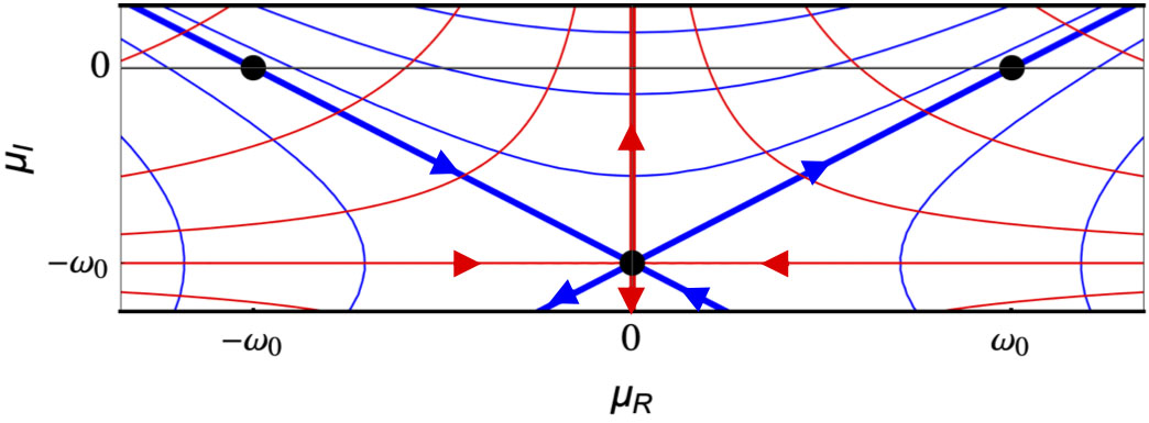
Figure 2: Elliptic (blue) and hyperbolic (red) contours for (2.1) and (2.2). The saddle at \((0,-\omega_0)\) is an organising centre for both the elliptic and hyperbolic contours. The stable and unstable manifolds of the saddle in (2.5) are the paths along which there is no exponential growth/decay of solutions. The stable and unstable manifolds of the saddle in (2.6) are the paths along which solutions have no rotation.

The elliptic contours (or Stokes lines) are the level curves of the Hamiltonian

\( \mathcal{H}_e = \operatorname{Re} \int_{\Gamma} \lambda(\tilde \mu)\, d\tilde \mu = (\mu_I+\omega_0)^2 - \mu_R^2. \)

As such, if \( \mu_0 \) and \( \mu\) are points on the real \(\mu\)-axis joined by an elliptic contour \(\Gamma_e\), then \( \operatorname{Re} \int_{\Gamma_e} \lambda(\tilde \mu)\, d\tilde \mu = 0 \). Since this integral is path independent, we may evaluate it along the real axis. This implicitly defines the way-in/way-out function [23, 24], \(\Psi\), such that

\( \int_{\mu_0}^{\Psi(\mu_0)} \operatorname{Re} \lambda(\tilde \mu)\, d\tilde \mu = 0. \)

Intuitively, the way-in/way-out function is the moment when the exponential repulsion on \(S_{\varepsilon}^r \) counterbalances the cumulative exponential contraction on \(S_{\varepsilon}^a \). Thus, solutions that start near \(S_{\varepsilon}^a \) at \( \mu_0\) will stay in a small neighbourhood of \(S_{\varepsilon}^r \) up to \( \Psi(\mu_0) \).

From Fig. 2, the only elliptic contours that join points on the real \(\mu\)-axis are those enclosed by the stable and unstable manifolds of the saddle at \((0,-\omega_0)\). Thus, \( \Psi(\mu_0) = -\mu_0\) for \(-\omega_0 <\mu_0 <0\), which is the memory effect. To use a financial analogy, the solution that starts at \(\mu_0\) builds credit as it tracks along \(S_{\varepsilon}^a\) and spends that credit once it starts tracking along \(S_{\varepsilon}^r\). Thus, the memory effect says that the credit spent (i.e., the time, \(\Psi(\mu_0)\), on the repelling manifold) is the amount of credit accumulated (i.e., the time, \(|\mu_0|\), spent on the attracting manifold).

For any \( \mu_0 < -\omega_0 \), the maximal elliptic contour that joins points on the real axis is the one consisting of the segment of the stable manifold of the saddle from \((-\omega_0,0)\) to \((0,-\omega_0)\) together with the segment of the unstable manifold of the saddle from \((0,-\omega_0)\) to \((\omega_0,0)\). Hence, \( \displaystyle \lim_{\mu_0 \to -\infty} \Psi(\mu_0) = \omega_0\) is the maximal delay that any solution can exhibit and is precisely the buffer point. (A rigorous proof of this was obtained in [23, 27] using adiabatic invariance theory and the method of stationary phase.) In the credit analogy, the buffer point is the maximum credit limit independent of how much credit has been accumulated.

Another useful characterisation of the memory effect and buffer point phenomenon can be obtained by studying (2.3) along hyperbolic contours (or anti-Stokes lines). These are the paths in the complex \(\mu\)-plane along which \( \operatorname{Im} \psi(\tau) \) is constant (Fig. 2), and are given by

\( \mu_R^\prime(\tau) = -\mu_R \\ \mu_I^\prime(\tau) = \mu_I + \omega_0. \)

(2.6)

The saddle equilibrium at \((0,-\omega_0)\) has a stable manifold along the line \(\{ \mu_I = -\omega_0\}\) and an unstable manifold along the \(\mu_I\)-axis. Since the vector field of (2.3) is analytic, integration along \(\{ \mu_I = -\omega_0\}\) is equivalent to integration along the real \(\mu\)-axis, by Cauchy's theorem. Transforming (2.3) along the hyperbolic contour \(\{ \mu_I = -\omega_0\}\) gives

\( z_s = \mu_R z + \sqrt{\varepsilon} I_a, \\ \mu_{R,s} = \varepsilon, \)

(2.7)

where \(s \) is such that \(ds = -\mu_R \, d\tau \). Thus, the rotation has been eliminated, and the nilpotent singularity at \( (z,\mu_R,\varepsilon) = (0,0,0) \) has been simplified.

To study the dynamics near the nilpotent point, the blow-up technique [9] (or geometric desingularization if you are working in public) is used. Blow-up consists of coordinate transformations that inflate the nilpotent singularity to a hypersphere and restore enough so that a complete analysis can be performed using standard dynamical systems techniques and center manifold theory.

For (2.7), blow-up is used to track \(z^a\) on \( S_{\varepsilon}^a\) forwards up to \( \{\mu_R = 0\}\), and \(z^r\) on \( S_{\varepsilon}^r\) backwards up to \( \{\mu_R = 0\}\). There, the distance, \(d\), between \(z^a\) and \(z^r\) at the saddle \( (\mu_R,\mu_I) = (0,-\omega_0) \) can be shown to be algebraically small. Then, \(d\) can be tracked along the hyperbolic contour corresponding to the \(\mu_I\)-axis, from the saddle \((\mu_R,\mu_I) = (0,-\omega_0)\) up to the bifurcation point \( (\mu_R,\mu_I) = (0,0) \). In doing so, it can be shown that the distance between the attracting and repelling slow manifolds at the bifurcation point is exponentially small

\( d = \left| z^a - z^r \right|= \left( \sqrt{2\pi \varepsilon} \left| I_a \right| + \mathcal{O}(\varepsilon) \right) e^{-\tfrac{\omega_0^2}{2\varepsilon}}. \)

The analysis of the distance measurement is presented in [16].

The distance between the attracting and repelling slow manifolds can be tracked past the bifurcation point by integrating along the real \(\mu\)-axis to give

\( d = \left( \sqrt{2\pi \varepsilon} \left| I_a \right| + \mathcal{O}(\varepsilon) \right) e^{\tfrac{1}{2\varepsilon} \left( \mu^2-\omega_0^2+2 i \mu \omega_0 \right)}. \)

It follows that, to leading order, the distance between \( S_{\varepsilon}^a\) and \( S_{\varepsilon}^r\) is exponentially small for \(\mu<\omega_0\), is \(\mathcal{O}(\sqrt{\varepsilon})\) for \(\mu \approx \omega_0\), and is exponentially large for \(\mu>\omega_0\). Thus, geometrically speaking, the buffer point is the location where the attracting and repelling slow manifolds diverge exponentially from each other.

2.3. The effects of nonlinear terms

For the nonlinear problem (2.1), the results from simplified Shishkova carry over. When \( \varepsilon = 0 \), (2.1) also has normally hyperbolic manifolds, which (recycling notation) we also denote by \(S_0^a\) and \(S_0^r\). For \(0<\varepsilon \ll 1\), these persist as attracting and repelling invariant slow manifolds, \(S_{\varepsilon}^a\) and \(S_{\varepsilon}^r\).

By studying the system either along the elliptic contours (as in [23, 24]) or along the hyperbolic contour \( \{\mu_I = -\omega_0\} \) (as in [16]), the dynamics of (2.1) are again analyzed in the neighbourhood of the saddle at \( (\mu_R,\mu_I)=(0,-\omega_0) \) in the complex \(\mu\)-plane. In either case, the nonlinearities make higher order contributions to the measurement of the distance between \(S_{\varepsilon}^a\) and \(S_{\varepsilon}^r\). Thus, at the Hopf bifurcation point \( \mu = 0 \), the distance can be shown to be exponentially small, i.e.,

\( d \leq \left( \sqrt{2\pi \varepsilon} \kappa + \mathcal{O}(\varepsilon) \right) e^{-\tfrac{\omega_0^2}{2\varepsilon}}, \)

where \(\kappa = \left| I_a \right| e^K \) for some \(K>0\). Consequently, the buffer point is still at \( \mu = \omega_0\) (to leading order) and is the location where the attracting and repelling manifolds diverge from each other. (Similarly, the memory effect of (2.2) persists in the full nonlinear problem (2.1) with small corrections.)

In other examples of delayed Hopf bifurcations in analytic ODEs, the nonlinear terms can play a more central role. For example, in [25] a quadratic nonlinearity changes the maximal delay estimate by an \(\mathcal{O}(\varepsilon \ln \varepsilon) \) amount.

3. Delayed Hopf Bifurcations in Reaction-Diffusion PDEs

Delayed Hopf bifurcation persists in reaction-diffusion PDEs. Among the earliest examples are [29, 30] in which the FitzHugh-Nagumo PDE is subject to a slowly varying applied current and weak periodic forcing. Further examples include singularly perturbed variants of Gierer-Meinhardt [32], Hodgkin-Huxley with slowly varying Neumann boundary condition [7], and cubic complex Ginzburg-Landau (CGL) with slowly varying parameter [21]. Rigorous analysis of pulses (and their delayed loss of stability) near supercritical HB in activator-inhibitor systems was presented in [33]. Most recently, the analysis of delayed bifurcations in PDEs that have infinite-dimensional fast subsystem (with spectral gap) and finite-dimensional slow subsystem was developed in [3]. It was shown that the FitzHugh-Nagumo PDE with slowly varying (and spatially uniform) parameter reduces to an ODE of the form (2.1) on the center manifold.

We will highlight some key features of delayed Hopf bifurcations in reaction-diffusion PDEs.

3.1. Cubic complex Ginzburg-Landau with source term

In [14], delayed Hopf bifurcations are studied in a spatially extended version of (2.1),

\( z_t = \left( \mu+i \omega_0 \right) z + \sqrt{\varepsilon} I_a(x)- \alpha \left| z \right|^2 z + \varepsilon D z_{xx}, \\ \mu_t = \varepsilon, \)

(3.1)

where \(\alpha \in \mathbb{C}\) is the nonlinear frequency, \(D \in \mathbb{C}\) is the linear dispersion, and \(I_a(x)\) is bounded and continuous. The initial data, \( z(x,0) = z_0(x) \) with \(\mu(0) = \mu_0\), is assumed to be bounded and continuous. (Equation (3.1) is the CGL equation with source \( \sqrt{\varepsilon} I_a(x) \) and slowly varying growth rate \(\mu\). We study (3.1) as an equation in its own right for \(\mathcal{O}(1)\) values of \(\mu\) and \(\omega_0 >0\).) Here, the source term and diffusivity are small-amplitude, however, the methods in [14] apply equally well for large-amplitude sources and diffusivities.

In the singular limit \(\varepsilon \to 0\), the \(z = 0\) state is stable for \(\mu<0\), unstable for \(\mu>0\), and undergoes a supercritical HB at \(\mu=0\). With \(0<\varepsilon \ll 1\), (3.1) has an attracting quasi-steady state (QSS) for all \(\mu < -\delta\), and a repelling QSS for all \(\mu > \delta\), where \(\delta>0\) is small and \(\mathcal{O}(1)\) with respect to \(\varepsilon\). Solutions converge to (diverge from) the attracting (repelling) QSS at an exponential rate. The attracting QSS (for \(\mu<-\delta\)) and the repelling QSS (for \(\mu>\delta\)) are given by

\( z_{\rm QSS} (x,\mu) = -\sqrt{\varepsilon} \frac{I_a(x)}{\mu+i\omega_0} + \varepsilon^{3/2} \left( \frac{I_a(x)+D(\mu+i\omega_0){I_a^{\prime \prime}}(x)}{(\mu+i \omega_0)^3} -\frac{(1+i\alpha)I_a^3(x)}{(\mu+i\omega_0)^2(\mu^2+\omega_0^2)} \right) + \mathcal{O}(\varepsilon^{5/2}). \)

Solutions in a fixed \( \mathcal{O}(1)\) neighbourhood of the attracting QSS (for \(\mu_0\) sufficiently negative) exhibit delayed loss of stability. These solutions approach the attracting QSS until they reach the instantaneous HB at \(\mu = 0\), and remain near the repelling QSS for long times before they escape the neighbourhood of the repelling QSS. Moreover, spatially decaying sources can balance the temporal exponential growth and hence the delay generally depends on the spatial position [14, 21]. An example is shown in Fig. 3.

Figure 3: Delayed Hopf bifurcation in (3.1) with \( I_a(x) = e^{-\tfrac{x^2}{4\sigma}}\). The solution starts left of the HB at \(\mu = 0\) (red line) and stays close to the attracting QSS (green background) for \(\mu<0\), and closely follows the repelling QSS for \(\mu>0\) until the black space-time buffer curve is reached. Beyond the space-time buffer curve, the solution diverges from the repelling QSS and oscillations set in.

3.2. Space-time buffer curve

Just as we saw for the simplified Shishkova ODE (2.2), it is also useful here to focus first on the linearisation of (3.1) about \(z=0\),

\( \varepsilon z_{\mu} = (\mu + i \omega_0) z + \sqrt{\varepsilon} I_a(x) + \varepsilon D z_{xx}, \)

(3.2)

assuming \( \mu_0 \leq -\omega_0\). The solution of this inhomogeneous heat equation consists of homogeneous and particular components, \(z_h\) and \(z_p\). To study these solutions, we analytically continue (3.2) into the complex \(\mu\)-plane and examine the solutions along elliptic and hyperbolic contours.

The behaviour of the solution in the complex \(\mu\)-plane depends on the form of the exponent

\( \psi(\mu) = \int_{\Gamma} \lambda(\tilde \mu) \, d\tilde \mu = -\tfrac{1}{2} \left( \mu_R^2 - (\mu_I+\omega_0)^2 \right) - i \mu_R (\mu_I + \omega_0) \)

(3.3)

where \(\lambda(\mu) = \mu+i \omega_0 \), and \(\Gamma = \mu_R+ i \mu_I\) is an integration contour. The elliptic and hyperbolic contours (or Stokes and anti-Stokes lines) for the CGL equation are identical to those of (2.1) and (2.3) (see Fig. 2). Using these contours, the particular solution can be tracked from the initial time \(\mu_0 \leq - \omega_0\), past the instantaneous Hopf bifurcation, and up to an \(x\)-dependent maximal value, \(\mu_{\rm stbc}(x)\), of \(\mu\) where \(z_p\) has unit magnitude. That is, \( z_p \) is exponentially small for \( \mu \in (\mu_0,\mu_{\rm stbc}(x)) \) and transitions to being \(\mathcal{O}(1)\) along \( \mu_{\rm stbc}(x) \). Thus, the space-time buffer curve [21] \( \mu_{\rm stbc}(x)\) is the maximal (to leading order) temporal delay that solutions with initial data at \(\mu_0 \leq -\omega_0\) can exhibit, and is the spatio-temporal analogue of the buffer point from ODEs. Examples of delayed Hopf bifurcation for various source terms, and their space-time buffer curves, are shown in Fig. 4 (see [21]).

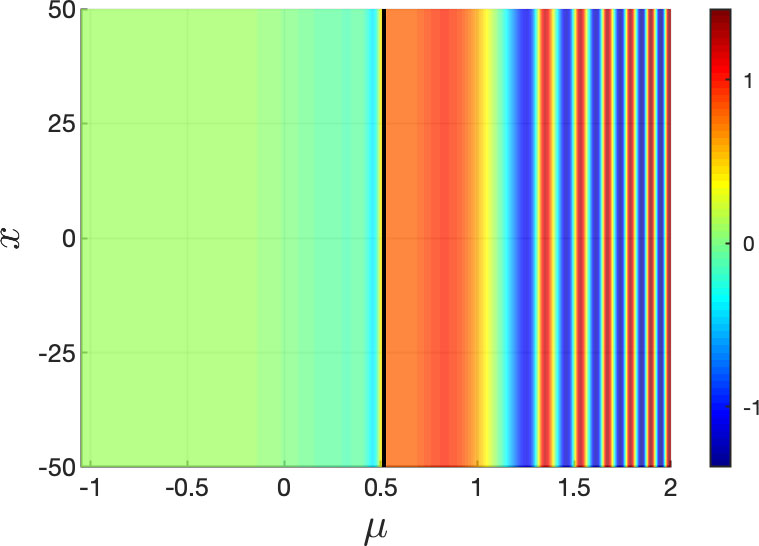
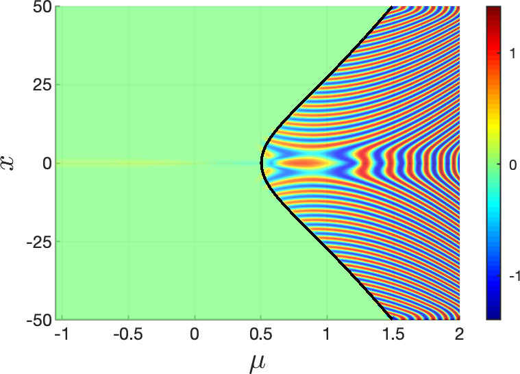
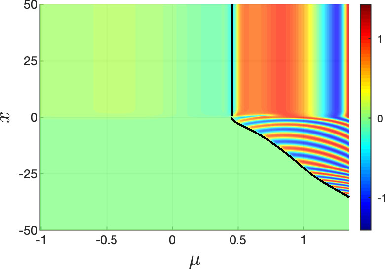
Figure 4: Simulations of (3.1) with zero-flux boundary conditions, and initial time \( \mu_0\) sufficiently large and negative. The source terms are (a) constant, (b) Gaussian (\( I_a(x) = e^{-x^2/(4\sigma)}\)), and (c) mollified step (\( I_a(x) = \tfrac{1}{2}(1+\tanh(x))\)) functions. Solutions stay close to the attracting and repelling QSS (green) until they reach the (black) space-time buffer curve, after which they oscillate. See [21] for details.

3.3. Competition between the homogeneous and particular solutions

There is a competition between which component, \( z_h(x,\mu) \) or \(z_p(x,\mu)\), first ceases to be exponentially small. The homogeneous solution transitions from being exponentially small to being \( \mathcal{O}(1)\) along the homogeneous exit time curve, \( \mu_h(x) \). Similarly, the particular solution transitions from being exponentially small to being \( \mathcal{O}(1)\) along the space-time buffer curve, \(\mu_{\rm stbc}(x)\). The spatial dependence of \( \mu_h(x) \) and \(\mu_{\rm stbc}(x)\) allows for different outcomes in the competition, resulting in distinct types of delayed Hopf bifurcations that depend on the time \( \mu_0\) at which the initial data is given, the form of the source term, and the system parameters. Full analysis of this competition, its outcomes, and important effects of the nonlinear terms are presented in [14]. Examples are illustrated in Fig. 5.

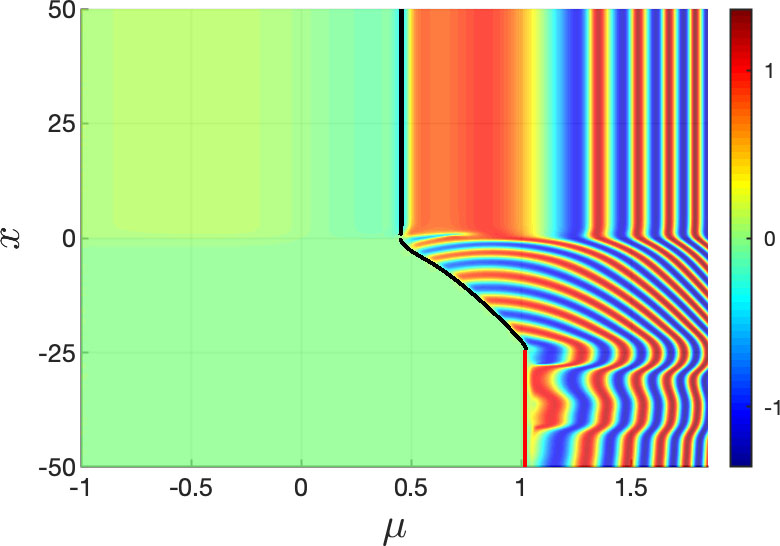
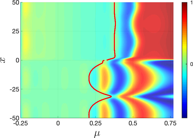
Figure 5: The delay in the CGL equation (3.1) is determined by the space-time buffer curve (black) and the homogeneous exit time curve (red). (a) For \(x \gtrsim -25\), the solution has maximal delay given by the space-time buffer curve. In contrast, on \(x\lesssim -25\), the homogeneous exit time curve occurs before the space-time buffer curve, so there is sub-maximal delay here and the oscillations set in at the same time on this subdomain. (b) With appropriately chosen initial data, \(\mu_h(x)\) occurs before \(\mu_{\rm stbc}(x) \) for all \(x\).

4. Outlook

Delayed loss of stability due to slow passage through Hopf bifurcations is a paradigm problem in dynamic bifurcation theory [6]. Two well-known results for delayed Hopf bifurcations in analytic ODEs, derived using elliptic and hyperbolic contours in the complex time-plane, are the memory effect and buffer points. The memory effect is the phenomenon in which the delay experienced by solutions depends on the amount of time spent following the attracting slow manifold. (This memory effect is symmetric in (2.1), i.e., \(\Psi(\mu_0) = -\mu_0\).) The buffer points have the geometric characterisation as being the points where the attracting and repelling slow manifolds diverge exponentially from each other. The buffer points are the maximal delay that any solution can experience, independent of how long it has spent on the attracting slow manifold, i.e., \(\lim_{\mu_0 \to -\infty}\Psi(\mu_0) = \omega_0\). The existence of buffer points depends on the symmetry-breaking source term \(I_a\) in (2.2).

In applications, the source terms \(I_a\) may vary in space, such as spatially localized applied currents in neuroscience and spatially localized light sources in chemical systems. This variation can induce spatially dependent delayed loss of stability due to slow passage through Hopf bifurcations. Such spatio-temporal delayed Hopf bifurcations have been demonstrated in a number of important reaction-diffusion PDEs, including Hodgkin-Huxley, FitzHugh-Nagumo, Gierer-Meinhardt, and cubic complex Ginzburg-Landau.

For CGL, the heart of the delayed Hopf bifurcation phenomenon lies in the competition between the homogeneous and particular solutions, to see which component first ceases to be exponentially small. As a result, the onset of oscillations is determined by the space-time buffer curve, \( \mu_{\rm stbc}(x) \), and the homogeneous exit time curve, \( \mu_h(x) \). Asymptotic formulas for these curves can be derived by studying the same elliptic and hyperbolic contours as in ODEs [14].

The field of dynamic bifurcations is an exciting area with many open questions. For instance, in the problems discussed here, the bifurcation parameter \(\mu\) has linear slow evolution. However, nonlinear slow evolution of \( \mu\) can substantially alter the delayed passage effects, as demonstrated in [5] for several key ODEs. The blow-up technique can be used to analyse these accelerating and decelerating ramps in ODEs. Such nonlinear ramps have yet to be studied in the PDE setting.

With one exception, delayed Hopf bifurcations in PDEs feature a slowly varying bifurcation parameter in the reaction kinetics. However, in applications, it may be of interest to study the PDE on a finite domain in which the slowly evolving parameter is injected via a boundary condition. Delayed Hopf bifurcation has been confirmed to exist in this setting [7]. Rigorous analysis of how the space-time buffer and homogeneous exit time curves are changed by the slowly varying boundary condition remains an open problem.

Delayed Hopf bifurcations and their associated way-in/way-out functions and buffer points are centrally connected to canard phenomenon [35]. Canards are solutions of singularly perturbed systems of ODEs that spend long times near an attracting slow manifold, pass through the neighbourhood of a fast subsystem fold bifurcation, and subsequently spend long times near a repelling slow manifold. The persistence of canards has been demonstrated in PDEs [1, 2, 8, 34]. With the recent advances in [3, 10, 18], there is much hope that the theory and applications of spatio-temporal bifurcation delay will lead to new spatio-temporal canard phenomena.

References

[1]   D. Avitabile, M. Desroches, E. Knobloch, and M. Krupa, Ducks in space: from nonlinear absolute instability to noise-sustained structures in a pattern-forming system, Proc. Roy. Soc. Lond. A, 473 (2017), 20170018.

[2]   D. Avitabile, M. Desroches, and E. Knobloch, Spatiotemporal canards in neural field equations, Phys. Rev. E, 95 (2017), 042205.

[3]   D. Avitabile, M. Desroches, R. Veltz, and M. Wechselberger, Local theory for spatio-temporal canards and delayed bifurcations, SIAM J. Math. Anal., 52 (2020), pp. 5703-5747.

[4]   S.M. Baer, T. Erneux, and J. Rinzel, The slow passage through a Hopf bifurcation: delay, memory effects, and resonance, SIAM J. Appl. Math., 49 (1989), pp. 55-71.

[5]   S.M. Baer and E.M. Gaekel, Slow acceleration and deacceleration through a Hopf bifurcation: Power ramps, target nucleation, and elliptic bursting, Phys. Rev. E, 78 (2008), 036205.

[6]   E. Benoît, Dynamic Bifurcations, Lectures Notes in Mathematics, 1493, Springer, Berlin.

[7]   L.M. Bilinsky and S.M. Baer, Slow passage through a Hopf bifurcation in excitable nerve cables: spatial delays and spatial memory effects, Bull. Math. Biol., 80 (2018), pp. 130-150.

[8]   P. De Maesschalck, T.J. Kaper, and N. Popović, Canards and bifurcation delays of spatially homogeneous and inhomogeneous types in reaction-diffusion equations, Adv. Differential Equations, 14 (2009), pp. 943-962.

[9]   F. Dumortier, Techniques in the theory of local bifurcations: blow-up, normal forms, nilpotent bifurcations, and singular perturbations, in D. Schlomiuk (Ed.), Bifurcations and Periodic Orbits of Vector Fields, in: NATO ASI Series C, 408, Kluwer, Dordrecht, 1993, pp. 19-73.

[10]   M. Engel and C. Kuehn, Blow-up analysis of fast-slow PDEs with loss of hyperbolicity, arXiv:2007.09973, 2020.

[11]   H. Engler, H.G. Kaper, T.J. Kaper, and T. Vo, Dynamical systems analysis of the Maasch-Saltzman model for glacial cycles, Physica D, 359 (2017), pp. 1-20.

[12]   T. Erneux, E. Reiss, L. Holden, and M. Georgiou, Slow passage through bifurcations and limit points: Asymptotic theory and applications, in Dynamic Bifurcations, Lectures Notes in Mathematics, 1493, E. Benoit (Ed.), Springer, Berlin, pp. 14-28.

[13]   N. Fenichel, Geometric singular perturbation theory for ordinary differential equations, J. Differential Equations, 31 (1979), pp. 53-98.

[14]   R. Goh, T.J. Kaper and T. Vo, Delayed Hopf bifurcation and space-time buffer curves in the Complex Ginzburg-Landau equation, arXiv:2012.10048, 2021.

[15]   X. Han, F. Xia, P. Ji, Q. Bi, and J. Kurths, Hopf-bifurcation-delay-induced bursting patterns in a modified circuit system, Comm. Nonlin. Sci. Num. Sim., 36 (2016), pp. 517-527.

[16]   M.G. Hayes, T.J. Kaper, P. Szmolyan, and M. Wechselberger, Geometric desingularization of degenerate singularities in the presence of fast rotation: A new proof of known results for slow passage through Hopf bifurcations, Indag. Math., 27 (2016), pp. 1184-1203.

[17]   L. Holden and T. Erneux, Slow passage through a Hopf bifurcation: From oscillatory to steady state solutions, SIAM. J. Appl. Math., 53 (1993), pp. 1045-1058.

[18]   F. Hummel and C. Kuehn, Slow manifolds for infinite-dimensional evolution equations, arXiv:2008.10700, 2020.

[19]   E.M. Izhikevich, Subcritical elliptic bursting of bautin type, SIAM J. Appl. Math., 60 (2001), pp. 503-535.

[20]   C.K.R.T. Jones, Geometric singular perturbation theory, in: R. Johnson (Ed.), Dynamical Systems, Montecatini Terme, in: Lecture Notes in Mathematics, vol. 1609, Springer, New York, 1994, pp. 44-118.

[21]   T.J. Kaper and T. Vo, Delayed loss of stability due to the slow passage through Hopf bifurcations in reaction-diffusion equations, Chaos, 28 (2018), 091103.

[22]   M. Krupa and M. Wechselberger, Local analysis near a folded saddle-node singularity, J. Differential Equations, 248 (2010), pp. 2841-2888.

[23]   A.I. Neishtadt, Persistence of stability loss for dynamical bifurcations. I, Diff. Eq., 23 (1988), pp. 1385-1391.

[24]   A.I. Neishtadt, Persistence of stability loss for dynamical bifurcations. II, Diff. Eq., 24 (1988), pp. 171-176.

[25]   A.I. Neishtadt, On calculation of stability loss delay time for dynamical bifurcations, in Proc. XI-th International Congress on Mathematical Physics, D. Iagoluitzer (ed.), 1994, International press, pp. 280-287.

[26]   J. Rinzel, Bursting oscillations in an excitable membrane model, in: B.D. Sleeman, R.J. Jarvis (Eds.), Ordinary and Partial Differential Equations, in: Lecture Notes in Mathematics, vol. 1151, Springer, Berlin, Heidelberg, 1985, pp. 304-316.

[27]   M.A. Shishkova, A discussion of a certain system of differential equations with a small parameter multiplying the highest derivatives, Dokl. Akad. Nauk SSSR, 209 (1973), pp. 576-579.

[28]   P. Strizhak and M. Menzinger, Slow passage through a supercritical Hopf bifurcation: Time-delayed response in the Belousov-Zhabtinsky reaction in a batch reactor, J. Chem. Phys., 105 (1996), pp. 10905.

[29]   J. Su, On delayed oscillation in nonspatially uniform FitzHugh Nagumo equation, J. Differential Equations, 110 (1994), pp. 38-52.

[30]   J. Su, Delayed bifurcation properties in the FitzHugh-Nagumo equation with periodic forcing, Differential and Integral Equations, 9 (1996), pp. 527-539.

[31]   D.X. Tran, D. Sato, A. Yochelis, J.N. Weiss, A. Garfinkel, and Z. Qu, Bifurcation and chaos in a model of cardiac early afterdepolarizations, Phys. Rev. Lett., 102 (2009), 258103.

[32]   J.C. Tzou, M.J. Ward and T. Kolokolnikov, Slowly varying control parameters, delayed bifurcations, and the stability of spikes in reaction-diffusion systems, Physica D, 290 (2015), pp. 24-43.

[33]   F. Veerman, Breathing pulses in singularly perturbed reaction-diffusion systems, Nonlinearity, 28 (2015), pp. 2211-2246.

[34]   T. Vo, R. Bertram, and T.J. Kaper, Multi-mode attractors and spatio-temporal canards, Physica D, 411 (2020), 132544.

[35]   M. Wechselberger, Canards, Scholarpedia, 2 (2007), 1356.