Handling editor: Steve Schecter

Donald G. Saari, Institute for Mathematical Behavioral Sciences, University of California, Irvine, CA 92697-5100, [email protected]

An ubiquitous sense of change runs throughout the social and behavioral sciences. Changes, after all, are observed everywhere; they occur in prices, in preferences for almost everything including consumer goods, in social customs and norms, in attitudes toward religion, in support for political candidates and public policies, in opinions, in needs of governance, and on and on. During the time when this article is being written, change is a particularly bothersome factor in our current economic struggle, as well as in the wild fluctuations in the stock market that promise to adversely affect our opportunities to retire at some time. Change is so fundamental and prevalent throughout the social and behavioral sciences that there is a clear need to model the underlying dynamics.

OK, so there is a need to model the dynamics. But how? A challenge confronting both the dynamical systems and social science communities is to find appropriate and useful modeling approaches. Quite bluntly, it is my opinion that much of the current modeling is not very good. To indicate my sense of what is needed, I'll identify a severe obstacle that hinders success: this obstacle reflects a fundamental difference between the social and physical sciences.

Those of us who have worked on the dynamics of physical systems are spoiled; we expect certain dynamical models to be able to predict with surprising accuracy. Way back in 1843, for instance, Le Verrier discovered that the perihelion of the planet Mercury (i.e., the position of Mercury's closest approach to the Sun) deviates 43 seconds of arc per century from that predicted by Newton's equations of motion. "43 seconds of arc?" As measured relative to the length of a football field, this is about 0.119 inches, or about the thickness of two pennies stuck together. That is precision!

While such accuracy may be expected in the physical science, it cannot be anticipated in the social sciences:

Even in economics, which is the most mathematical of the social sciences, no one really believes that a prediction could be made with even 10% accuracy of the actual value of some economic feature, say the stock market, for a year from today - leave alone predicting its value for a century from now. Indeed, I doubt whether there were any professionals who made even a roughly accurate economic prediction during the summer of 2008 about what would hit us only months later.

What is being done in these areas? Probably as a result of trying to mimic and capture the success of the physical sciences, models of change in the social and behavioral sciences tend to adopt the standard form of

x'=f(x) (1)

where f(x) captures behavioral interactions. Some of these models have provided useful insights, but I worry whether the Eq. 1 form is an appropriate choice for these areas. After all, it is disturbingly easy to identify many papers for which, after much difficult work, deep results are obtained about an Eq. 1 type of equation - that nobody really believes or accepts. Indeed, with all of the vagueness and differences that characterize interactions within the social sciences, it is difficult to believe that any single equation can adequately capture what is actually happening. A challenge for the dynamical systems and social science communities, then, is to help to resolve this problem where we do not fully understand how to adequately model change in these disciplines.

Quite often the best that can be expected in the social sciences is a qualitative prediction. While such an objective suggests using probabilistic and related approaches, this methodology is unsatisfactory for many issues. After all, the problem is not one of randomness; it is that we really do not understand how to model behavior and the associated changes. Not much help in creating appropriate models comes from current dynamical systems literature; this is because many of these results reflect the kind of dynamics that arise in the physical sciences where an emphasis is placed on precision. A challenge, then, is to find ways to appropriately model "qualitative" social dynamics.

The surprising complexity of price dynamics

Adam Smith, 1723-1790. The economic theories of Smith rely on the existence of a market global attractor.

In the modeling of social science dynamics, careful attention must be paid to their established structures. For instance, in certain social sciences, such as in economics, there can be wide agreement about the nature of the equilibria of the dynamics even though there may be very little understanding, leave alone consensus, about the actual dynamics.

Leon Walras, 1834-1910. Walras' classical Laws of Economics identify three important properties of "supply and demand," or the aggregate excess demand function.

An illustrating example comes from a freshman course in economics that introduces the Walrasian equilibrium. This equilibrium is a price vector

p =(p₁, ..., p_c)
(one price for each of the c>1 commodities) where the "markets clear"; stated in words, at these prices the supply of each commodity equals its demand. But while the equilibria are well defined, the appropriate price dynamic remains a deep mystery even for a highly idealized "pure exchange economy" setting. This is where, rather than producing or consuming anything, the a>1 economic agents merely exchange goods.

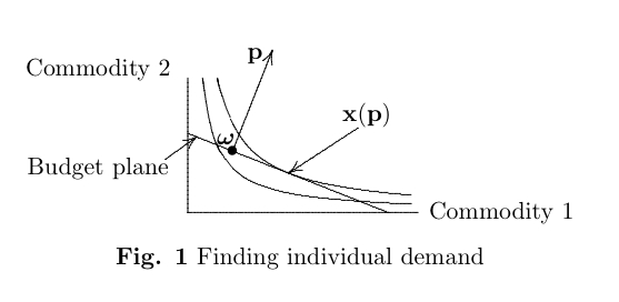
Presumably the price changes in such an economy, as given by p', are based on market pressures as captured by the economy's aggregate excess demand function ξ(p). This function is the difference between the sum of individual demands for each good minus the sum of what will be supplied at the p prices. For a primer how to find ξ(p) (Fig. 1), let vector ω_j represent the j^th agent's initial allocation; ω_j specifies the (positive) amount of each commodity possessed by this agent. At prices p, the worth of ω_j is given by the scalar product p ⋅ ω_j. By selling (hence supplying) some of these holdings, the agent can afford to buy any commodity bundle x_j where

p ⋅ ω_j = p ⋅ x_j, or p ⋅ [x_j - ω_j] = 0. (2)

As the plane p ⋅ [x_j - ω_j] = 0 in R₊^c (space of commodities) describes what this agent can afford at prices p, it is called the budget plane.

Herbert E. Scarf, Professor of Economics, Yale University. Scarf was the first to describe a case in which the dynamics near an economic equilibrium were repelling, indicating the complexity of price dynamics in economics.

It remains to determine what the agent wants. A standard approach used to characterize an agent's preferences, which cuts across the social and behavioral sciences, is to impose an order on R₊^c by borrowing from the complete and transitive ordering of the real line. This is done with a utility function

U_j:R₊^c → R¹;

when comparing two commodity bundles, the agent prefers the one with the larger U_j value. Similarly, the U_j level sets, which are called indifference surfaces, consist of the commodity bundles over which the agent is indifferent.

To further simplify the analysis, U_j usually is assumed to be a convex (i.e., concave up) continuous function. For convenience of analysis, U_j often is further assumed to be a smooth function. With this structure, finding what the agent wants reduces to a Lagrange multiplier exercise of determining the unique (recall, U_j is convex) x_j(p) that maximizes U_j subject to the Eq. 2 budget constraint. Notice how the answer provides economic intuition; the positive and negative components of the individual excess demand function ξ_j(p) = x_j(p) - ω_j represent, respectively, what this agent demands and is willing to supply at prices p. The Fig. 1 agent, for instance, is willing to sell some of commodity 2 to obtain enough money to purchase more of commodity 1.

The aggregate excess demand function is the sum of the a individual excess demands

ξ(p) = \(\Sigma_{j=1}^a\) ξ_j(p). (3)

This is the stage where dynamics step in. For instance, the standard Adam Smith's "invisible hand" story suggests that the price dynamic is given by

p' = ξ(p), (4)

or, in a discrete form, by

p_n+1 = p_n + ξ(p_n). (5)

Both expressions require prices to increase and decrease according to market pressures; i.e., prices for commodities that are associated with positive components of ξ(p) increase (as the demand is greater) and decrease for goods with negative components.

The traditional Adam Smith story is that the market pressures always lead to an equilibrium. Restated in terms of dynamical systems, Smith believes that the price dynamic has a global attractor that is an equilibrium. At least with all of these simplifying assumptions, this belief seems to be plausible. But is it? Is the story correct even in this highly simplified setting? In order to examine this issue, we need to know the properties of the dynamic, starting with the stability of the equilibria where

ξ(p^*) = 0.

The derivation of ξ(p) makes it clear that all properties of the dynamics derive from the choices of the utility functions. Herein lies a problem that cuts across the social sciences: Which selection is an appropriate one? With a function space of possible choices, it is reasonable to worry whether different selections could cause radically different dynamics --- even though all utility functions satisfy the desired assumptions.

The first to explore this possibility was Herb Scarf [12]. Scarf created a simple but clever example of a three-person, three-commodity economy with a unique ξ(p) equilibrium, but the equilibrium is a repeller; i.e., with the Eq. 4 dynamic, prices can never reach this equilibrium. Instead, the prices in Scarf's economy are doomed to cycle forever while approaching an attracting periodic orbit.

Scarf's conclusions were significantly extended by Sonnenshein [13], Mantel [7], and Debreu [2]. Their combined effort led to a theorem that uses the standard properties of ξ(p) (called Walras' laws, which are listed in the Reference section[1]) and imposes a minor technical constraint (that the prices for these desired goods are bounded as slightly away from zero as desired). The SMD Theorem asserts that if a≥ c, then any continuous function F(p) satisfying these conditions is the aggregate excess demand function for some pure exchange economy!

The kicker of this result is that no matter how wild the choice of F(p), no matter how chaotic the resulting Eq. 4 or Eq. 5 price dynamic, no matter how grossly the choice of F(p) violates any common sense attitude about economics, as long as a≥ c there exists a pure exchange economy (i.e., each agent is assigned an initial endowment and an appropriate utility function) so that ξ(p) = F(p)! As the SMD theorem allows an economy's aggregate excess demand to be almost anything, no real constraints can be imposed on the Eq. 4 behavior; the dynamic can be as wild and chaotic as desired. While this assertion sounds outrageous, when viewed in light of the current economic behavior, maybe this theoretical assertion supplies some lessons.

My extension of this result (Saari [9]) is even more troubling. It asserts that for each subset of two or more commodities, you can select any continuous function satisfying Walras' laws; let the choices differ as wildly as desired. The conclusion is that, with the same constraint on prices and for an "a" value such that a≥ c, there exists an economy such that, for each of the 2^c-(c+1) subsets of goods, if we consider the "subeconomy" having only the goods in that subset, the selected function is the subeconomy's actual aggregate excess demand function.

In other words, the act of adding or eliminating a commodity can generate highly unexpected market consequences. This assertion makes sense; just recall how introducing the office copier, the cell phone, or the ipod, changed the economics of supply and demand. But this theorem also means, for instance, that it is possible to create an economy where the Eq.5 price dynamics for the set of three commodities is well behaved with a global attractor even though the Eq. 5 price dynamic on each of the three sets of two commodities is as chaotic as desired!

All of these problems makes it reasonable to wonder whether the price dynamic is something other than that of Eq. 4. It is reasonable to wonder whether a more accurate choice reflects some unknown economic process that massages the ξ(p) market information in an appropriate manner to assume the form of

p' = M(ξ(p)) (6)

where M is a continuous function. The key problem, of course, is to find the appropriate choice of M. But when Carl Simon and I explored this question [10], we adopted the spirit of this current article by deciding not to concentrate on what happens with a single model or dynamic, but to explore what can happen with all possible choices of M over all possible economies. The advantage of doing so was our discovery that no such M exists; instead, we showed for any choice of M that there is an open set (in almost any topology) of economies and an open set of initial conditions for which the Eq. 6 dynamic fails to converge! We also found that in order to design a universal mechanism that will always converge to an equilibrium, the price mechanism must use all of the information from ξ(p), almost all from the Jacobian Dξ(p), and global (index) information about the structure of the economy. That is a considerable amount of information! I am not sure whether it is realistic to assume that "real systems" can incorporate and process all of that data.

But even after creating such a p'=M(ξ(p), Dξ(p)) system that does converge to some equilibrium, the fact the model requires a continuous change of p suggests that an infinite amount of information is being smuggled into the analysis. Namely, p' expressions are natural for the physical sciences where, say, rather than taking time off to have dinner, to go to sleep, or to stop for a cup of coffee, astronomical bodies continually pull on each other. But it is not clear what these instantaneous changes means when differences are being determined by human decision processes. As such, it is reasonable to explore what happens to prices with a discrete dynamic of the Eq. 5 form.

The difficulties become much worse! Again my adopted approach was to determine what can happen in general rather than in specific cases. As I showed (Saari [8]), even if schemes are carefully designed to use the market pressure story, even if past market information involving as many derivatives as desired is included in a manner so that the dynamic assumes the form

p_n+1 = p_n + M(ξ(p_n), ..., ξ(p_n-k), ..., D^jξ(p_n), ..., D^jξ(p_n-k)) (7)

where k and j are any specified positive integers, there always exists an open set of initial conditions and of economies where the dynamics need not even get close to any equilibria.

This negative result suggests that the usual "invisible hand" stories probably require using an unrealistic infinite amount of information. Or, maybe the result suggests that we should search for new ways to model price dynamics.

As a footnote, notice how this negative assertion about the choice of an M for Eq. 7 includes the higher dimensional Newton iterative process. The assertion even includes global Newton methods that do converge. The key difference is that in price dynamics, the initial conditions cannot be required to lie in a particular region; they are what they are. In contrast, the initial conditions for global Newton methods are required to be in specified regions, usually on the boundary, in order to incorporate global index properties.

What else?

As this brief description makes clear, characterizing when an equilibrium is an Eq. 4 attractor requires using the aggregate properties of the utility functions. But, we don't know which functions are the appropriate choices, and a difference in the choice can make a difference in the price dynamics. It is, of course, possible to extract results about classes of choices. For instance, by invoking the inverse function theorem and using the relationship between the slopes of the function and its inverse, it becomes clear that a price equilibrium will be unstable if, in some sense, the aggregate of the utility functions is overly flat at an equilibrium price. But even should a specific equilibrium be shown to be an attractor, the properties of the basin of attraction remain captive to the choice of the utility functions. In other words, it is not clear what can be said in general.

Maybe we should abandon the search for a universal price mechanism; maybe we should concentrate on finding what happens for specific subsets of economies. I doubt, for instance, whether anyone really expects the markets of Los Angles, Rio de Janeiro, and Calcutta to behave in the same manner. This intuition has theoretical support; it turns out (Saari and Williams [11]) that there exists a finite number of different matrices M where each is associated with a particular subset of economies; only a small set of economies are excluded from this story. The property is that the price mechanism defined by each M choice (when applied to an economy from its associated set) allows at least a locally converging Eq. 6 price behavior (Saari and Williams [11]). But this conclusion is primarily an existence result; the pragmatic issue of finding ways to connect matrices to a set of appropriate economies remains essentially unexplored.

Even if answers for the above concerns can be found, my sense is that the actual problem remains far more complicated and severe. My worries reflect the reality that there is a function space of choices for the utility functions. Until a realistic way can be found to capture the precise utility functions that apply for particular economies, I remain skeptical about predictions and results that are based on specified choices of ξ(p). Stated in other words, there is a need to create a qualitative dynamical approach to describe what happens for classes of economies. This is not a structural stability issue with its goal of determining whether the dynamics remain essentially the same when subjected to small but unknown perturbations. The goal is to determine what can be expected to happen with relevant classes of dynamics; part of the challenge is to determine the meaning of "relevant."

The reason I selected this price mechanism story to describe my concerns about the modeling of dynamics in the social sciences is that, with this story, it is easy to understand the source of the complexity. Namely, when trying to understand what happens in general, the modeling must emphasize a function space of utility functions, rather than special cases. Currently, however, we don't know how to handle this challenge even in the described simplified setting.

The problem is not restricted to price dynamics, nor even to economics. Instead, across the social and behavioral sciences, utility functions are commonly used to characterize individual preferences and the subsequent actions. This means that even if we understand the goals and objectives of the dynamics for these social science areas, which is true with the price equilibrium story, for many of these areas we still do not understand the behavioral properties that define the dynamics. As such, we should treat most results that are based on a specific dynamical equation as specifying what can occur in some highly specialized setting; I cannot accept such conclusions as realistically indicating what to expect in general. New ways to capture the general qualitative behavior are required.

Darwin and altruism

February 12, 2009, marked the 200^th anniversary of Charles Darwin's birth. A puzzle about his "On the Origin of the Species" involves the unmistakable existence of altruism. How and why can it evolve and occur?

This altruism mystery is but one of several topics that are of interest in evolutionary game theory (e.g., Hofbauer and Sigmund [5,6]). It is reasonable to view this area as the wedding between dynamical systems and game theory, which probably explains why this approach is attracting more and more interest in the social and behavioral sciences. To explain this connection in terms of an example, let me describe the Ultimatum Game.

This "single-shot" game has two players; while both know the rules, they do not know who is the other player. The first player is given a sizable amount of money, say $1000. The rules require her to share some of this cash with the other, unknown player. After she specifies how much she will offer the second player, he makes the final decision. If he agrees, he receives the offered amount and she keeps the rest. But if the second player refuses, both get nothing. How much should the first player, or would you, offer?

The standard answer coming from game theory is to offer a single dollar. After all, it remains in the second player's best interest to accept this paltry amount because, by doing so, he ends up with more money than if he refuses. However, in experiment after experiment, the second player refuses to cooperate unless the dollar amount is at least around 40% of the total. While answers can change when this experiment is run in different cultures (Henrich et. al. [4]), the classical game theoretic solution of a dollar fails to hold. Why? What is happening?

Clearly, the experiments capture some behavioral feature that goes beyond the traditional game theoretic modeling of this situation. There is a distinct sense that the explanation involves social norms; e.g., different cultures have different standards of when you feel you are being cheated. The associated question, then, is to understand how societal expectations evolve; here dynamics play a central role (e.g., Skyrms [14]). The standard approach is to identify the k kinds of actors in terms of a vector x = (x₁, ..., x_k) ∈ R^k where x_j represents the proportion of the total population that is of the j^th type. Next, write down the game theoretic interactions and reactions among the players in an Eq. 1 format. In this manner, which mimics some of the theoretical research involving the dynamics of evolutionary biology (e.g., Frank [3]), answers are forthcoming.

Let me confess that I am a big fan of evolutionary game theory along with its explanations about, for instance, the central role of punishment in creating an orderly society. But my earlier criticism remains. My sense is that social science results that are based on specific choices of x'=f(x) must be treated as existence theorems. These results should be welcomed as providing insight by establishing that settings exist in which the specified kind of outcome occurs; may it involve altruism, greed, reciprocity, or something else. But with this modeling, I cannot accept the conclusions as providing a general explanation of what is happening with the same confidence that I can assign to models from the physical sciences.

It is my sense that to advance these areas, we need to find ways to model the wider spectrum of possibilities that occur in the social and behavioral areas. Currently I am developing one approach, but it is limited in nature; a more general effort is required. I offer this description and problem as a challenge to the dynamical systems community.

Intuition behind certain proofs

The purpose of this concluding section is to provide intuition about some of the conditions in the above theorems and how certain of them are proved. Let me warn you, I am taking considerable liberties in this description as my emphasis is on intuition; the approach of the actual proofs can differ (check them for details).

SMD Theorem. To prove the SMD result, reduce by one the dimension of the problem. This is done by using the Walras condition that, for a positive scalar λ, F(λp) = F(p). This homogeneity property coupled with Walras' condition p ⋅ F(p)=0 allows F(p) to be viewed as a tangent vector field on the price simplex, which is a portion of the unit sphere

{p | Σ\(_{j=1}^c\) ( p_j²) = 1, p_j>0 }.

The minor technical condition imposed on the prices is that, for any ε>0, only prices in the price simplex that satisfy p_j≥ ε for j=1, ..., c are considered. A purpose of this condition is to avoid problems near the simplex's boundary.

As F(p) is to represent an aggregate excess demand function, it can be expressed as

F(p) = Σ\(_{j=1}^a\) F_j(p)

where each F_j(p) is another tangent vector field on the price simplex; F_j(p) represents the j^th agent's excess demand function. In the standard way, a point in the price simplex (of dimension c-1) can be expressed as a convex combination of the c vertices. Similarly, if each vertex is assigned a vector that points inward, then any other given vector can be represented with a similar convex combination. To capture this effect with individual excess demands, if there are at least as many agents as commodities (this is the source of the a≥ c condition), assign the initial endowment to the j^th agent with an abundance of the j^th commodity but limited amounts of the other goods. In this manner and for any price, the agent's aggregate excess demand points away from the plentiful commodity and toward some combination of the others. Of mathematical importance, if a≥ c, then any vector, including F(p), can be expressed as a convex combination. Using this approach and taking advantage of the cancellation effects of a summation, the F_j(p) functions can be selected to have fairly "nice" properties.

We still need to find the utility functions. Returning to Fig. 1, notice that at each p, the F_j(p) function represents only one tangent direction at x_j(p) and that there is some freedom in selecting x_j(p). This fact suggests using the Frobenius Theorem from differential geometry to define an appropriate foliation for each agent; the leafs represent the level sets of the j^th agent's utility function. The ultimate goal, however, is to have a continuous foliation. To achieve this objective, technical approaches other than the Frobenius Theorem need to be developed. While this creates a more difficult analysis, all of this can be done.

My extension of the SMD Theorem. My extension of the SMD assertion to all subsets of two or more commodities is based on two observations. The first is that, with a gi