A basic first step in the analysis of a singularly-perturbed system is the identification of its locally invariant slow manifolds, together with their associated fast fiber bundles. We are concerned with \(n\)-dimensional systems of ODEs of the general form

\( z' = H(z,\epsilon), \)

(0.1)

where the parameter \(0 \leq \epsilon \ll 1\) characterizes, for instance, a ratio of timescales in the underlying dynamical processes. Such a family defines a singular perturbation problem if there exists a \(k\)-dimensional critical manifold \(S \subset \{z \in \mathbb{R}^n: H(z,0) = 0\}\) of equilibria, where \(1 \leq k < n\). For simplicity we take \(S\) to consist of a single connected smooth component, although more complicated configurations are possible; for example, critical sets consisting of intersecting varieties arise in biochemical models, and analysis of the flow near the `corners' can play a crucial role in reconstructing the global dynamics (see for e.g. [9]).

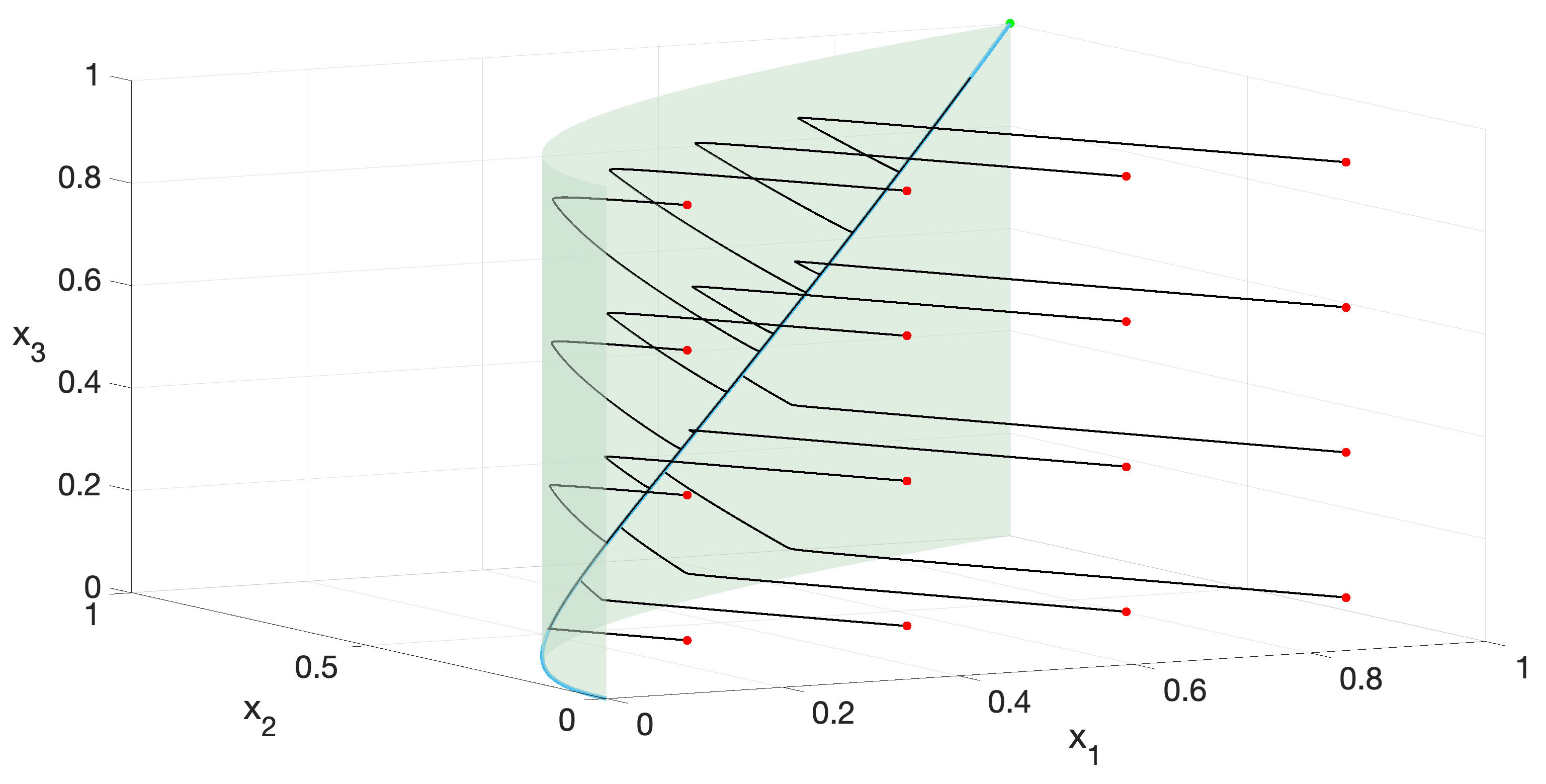
Figure 1. Dynamics of a singularly-perturbed dynamical system \(z' = H(z,\epsilon) = h_0(z) + \epsilon h_1(z) + \epsilon^2 h_2(z)\) modeling a hypothetical three-timescale reaction network, with \(\epsilon = 0.01\). Trajectories with initial conditions specified by the red points quickly settle near a critical surface, before slowly drifting toward the light blue curve. The dynamics on the curve is `infra-slow.' See [15] for details.

A celebrated---and by now rote---result of Fenichel [3] describes how invariant slow manifolds and fast fiber bundles emerge as smooth perturbations of their singular counterparts under \(\epsilon\)-variation. These objects in turn provide a geometric `skeleton,' organizing nearby solutions. This result is a cornerstone of geometric singular perturbation theory (GSPT) (see for eg. [11, 18] for exhaustive expositions). There has been very recent progress made on extending these classical results to the case of more than two timescales [1, 10], but the story is far from complete. Figure 1 depicts the dynamics of a representative three-timescale system.

We can rephrase Fenichel's fundamental result in a way that emphasizes its computational content: the `singular' objects, defined for \(\epsilon = 0\), are the leading-order approximations to the slow manifolds and fast fibers. Rigorous analysis of the slow and fast objects typically requires knowledge of the higher-order terms in their corresponding asymptotic expansions (in orders of \(\epsilon\)). This leads us to our primary question:

How do we approximate the slow manifolds and fast fibers, analytically or numerically, to arbitrary order in \(\epsilon\)?

Let us attempt to formulate the problem more precisely, at least for slow manifolds in two-timescale problems. Suppose that the critical manifold \(S\) is locally expressible as a graph over some choice of slow variables \(x \in U \subset \mathbb{R}^k\):

\( S|_U := \{(x,h_0(x)) \in S: x\in U\}. \)

Our goal is to compute an asymptotic expansion for the slow manifold \(S_{\epsilon}\) nearby:

\( S_{\epsilon}|_U := \{(x,h_{\epsilon}(x) = h_0(x) + \epsilon h_1(x) + \cdots + \epsilon^k h_k(\epsilon) + \cdots) \in \mathbb{R}^n: x \in U\}, \)

i.e. we seek iterative formulas for the higher-order terms \(h_{i \geq 1}\) in terms of the derivatives of \(H\) and \(h_0,\cdots,h_{i-1}\). We remark here that the slow manifolds are nonunique but are \(O(e^{-c/\epsilon})\)-close (for some \(c = c(H|_V) > 0\), where \(V\) is a compact set containing \(S|_U\)), so the asymptotic series is well-defined.

The apparent dependence of the solution on an explicit choice of coordinates is undesirable. We point out that the system (0.1) need not be written over a global coordinate chart specifying slow versus fast variables, and finding analogous local transformations can be complicated. This step is taken for granted for systems written in the more restrictive standard form

\( \begin{array}{rl} &x' =\epsilon g(x,y,\epsilon)\\ &y' = f(x,y,\epsilon). \end{array} \)

(0.2)

There are many contexts in which this kind of global splitting is too artificial, since slow versus fast processes are typically identified rather than slow versus fast variables. One can usually hope that systems of the form (0.2) will correspond to rescalings of (0.1) in locally-defined regions of the extended phase space. These observations motivate the development of coordinate-independent algorithms to approximate slow manifolds and fast fibers.

In this article we explore two such algorithms: the computational singular perturbation method [12, 13, 14] and a new type of parametrization method [15]. The point of view we want to emphasize is that a careful study of the intrinsic geometry of (0.1) not only naturally motivates each iteration scheme, but also clarifies `for free' why they both enjoy the property of coordinate independence. For the parametrization method, this geometric emphasis turns out to be particularly fruitful: we show that we can extend the method to tackle multiple-timescale problems, i.e. where more than two distinct timescales feature in the dynamics, as in Figure 1.

1. Computational singular perturbation (CSP) method

The CSP method is a popular approximation scheme developed by Lam and Goussis [12, 13] to study model reduction of chemical reactions. The geometric content of the method has since been explored in depth and rigorous convergence theorems have been proven [6, 7, 8, 16, 17]; we relate some of these results here. The iteration step is motivated by understanding how the system (0.1) augmented by the variational equations (i.e. the dynamics on the tangent bundle \(\simeq \mathbb{R}^{2n}\)) transforms under smooth coordinate transformations, when restricted to an invariant manifold. The CSP method seeks to identify the `simplest possible' coordinates to describe invariant manifolds and their transverse fiber bundles.

Let \(A(z)\) denote a smooth \(n\times n\) matrix which is regular for each \(z \in S_{\epsilon}\), and let \(B(z)\) denote its dual. Expressing the vector field \(H\) in the new basis

\( g(z) = B(z) H(z), \)

it turns out that the variational equation transforms according to the action of a Lie bracket, namely

\( g' = B[A,H]g. \)

The Lie bracket \([A,H]\) is defined in the `natural' way, i.e. columnwise in \(A\). The key observation that links this geometric fact with a computational method is that the operator

\( \Lambda = B[A,H] \)

can be block-diagonalized if the (point-dependent) matrix \(A\) is chosen `cleverly.' In fact the clever choice is the natural one: we have an invariant manifold with a transverse fiber bundle, so at each point \(z \in S_{\epsilon}\), we select the columns of \(A\) as follows:

\( A(z) = \begin{pmatrix} A_f(z) &  A_s(z) \end{pmatrix}, \)

(1.1)

where the image of the \(n\times (n-k)\) matrix \(A_f\) spans the transverse fibers \(F_{\epsilon,z}\) and the image of the \(n\times k\) matrix \(A_s\) spans the tangent space of \(S_{\epsilon}\), according to the splitting

\( T_z\mathbb{R}^n = F_{\epsilon,z} \oplus T_z S_{\epsilon}. \)

Such splittings are assured in the case of normally hyperbolic critical manifolds. The block structure of \(A\) induces a corresponding block structure of its dual \(B\):

\( B(z) = \begin{pmatrix} B_{s\perp}(z) \\ B_{f\perp}(z) \end{pmatrix} \)

The slow manifold and fast fiber bundle can be easily expressed in terms of \(B_{s\perp}(z)\) resp. \(A_f(z)\).

Of course, if we knew \(S_{\epsilon}\) and \(F_{\epsilon}\) already we would be done; instead we only know the leading order approximations \(S\) and \(F\). We now ask for a method which, given an initial guess for a splitting \(A^{(0)}(z)\) (whose block columns span \(F_z\) and \(T_z S\), respectively, along points \(z \in S\)), produces a sequence of matrices \(A^{(0)}(z), A^{(1)}(z), \cdots\) so that for each \(i\), the corresponding variational operator

\( \Lambda^{(i)}= B^{(i)}[A^{(i)},H] \)

is `more block-diagonalized' than the preceding operators in the list. The idea is that the pair \((A^{(i)},B^{(i)})\) that does the job can generate \(O(\epsilon^i)\)-close approximations of the slow manifold and fast fiber bundle. Zagaris, Kaper, and Kaper proved several convergence theorems of the following type across a very detailed set of papers [6, 7, 8].

Theorem 1.1. [6] At a given iteration step \(j \geq 0\), any asymptotic expansion of the `CSP manifold of order \(j\)' \(K^{(j)}_{\epsilon}\) agrees with the corresponding expansion of the slow manifold \(S_{\epsilon}\) up to and including \(\mathcal{O}(\epsilon^j)\) terms.

Let us now describe the actual iteration step. A remarkable feature of the CSP iteration is that near-identity transformations suffice for convergence (in the sense of the preceding Theorem). Near-identity maps are not only relatively efficient to compute numerically; they are also easy to invert. This is crucial, because we require the duals \(B^{(i)}\) (specifically, the first block row of \(B^{(i)}\)) in order to approximate the slow manifold. The two-step CSP method is

\( \begin{array}{rl} &A^{(i)} \mapsto A^{(i+1)} = A^{(i)} (I-U_i)(I+L_i)\\ &B^{(i)} \mapsto B^{(i+1)} = (I-L_i)(I+U_i)B^{(i)}, \end{array} \)

where \(I\) denotes the \(n\times n\) identity matrix and \(L_i,U_i\) denote, respectively, block lower- and upper-triangular nilpotent matrices. The nonzero block components of \(L_i\) and \(U_i\) are defined so that the method converges. A simple choice turns out to depend on block components of \(\Lambda^{(i)}\).

Note that the two-step method involves computing two near-identity transformations, corresponding to updating both block columns (resp. block rows) of \(A^{(i)}\) (resp. \(B^{(i)}\)). Thus we refine our approximations of the slow manifold and the fast fibers simultaneously at the end of each iteration. If we are interested only in slow manifold approximations, a corresponding one-step method can be used to update only the first block column of \(A^{(i)}\) (resp. the first block row of \(B^{(i)}\)). One-step versus two-step variants also arise in the parametrization method.

We initialize the CSP method by first identifying (point-dependent) bases for the tangent space and the transverse fast fiber bundle of the critical manifold \(S\). Let

\( H(z,\epsilon) = H_0(z) + \epsilon G(z,\epsilon). \)

Information about the geometry near to the critical manifold \(S \subset \{z \in \mathbb{R}^n: H_0(z) = 0\}\) can be obtained from the eigenvalues and eigenvectors of \(DH_0\). The eigensystem can be numerically calculated very efficiently. On the other hand, there are many families of systems for which

\( H_0(z) = N(z)f(z), \)

where \(N(z)\) is a matrix having full rank along \(S\). This factorization can be interpreted as a stoichiometric weighting in models of chemical reaction networks [5]; in the case of rational vector fields, they can be even be (locally) constructed explicitly [4]. This factored form turns out to be convenient for initializing the method, because \(N\) and \(Df\) provide information about the tangent space and fast fibers near normally hyperbolic critical manifolds [14, 18]. Taking our cue from the `clever' choice (1.1), we select the initial condition

\( \begin{align*} A^{(0)}(z) &= \begin{pmatrix} A_f(z) & A_s(z)\end{pmatrix} \\ &= \begin{pmatrix} N(z) & P(z) \end{pmatrix}, \end{align*} \)

where \(P(z)\) is any matrix whose columns span the kernel of \(Df\). With this initialization, further iterations of the method can be written in terms of derivatives of \(N\), \(f\), and \(G\) giving effective formulas. For example, suppose we choose any chart so that the slow manifold is locally given by

\( y = h_0(x) + \epsilon h_1(x) + \mathcal{O}(\epsilon^2). \)

The CSP method then gives an explicit formula for the first-order correction:

\( h_1 = -(D_y f)^{-1} (D\!fN)^{-1} (Df\,G). \)

We can derive similar kinds of formulas for the fast fiber bundle. We emphasize that we selected a representation here only for convenience; the convergence is coordinate-independent. Factorizations of the form \(H_0 = Nf\) obviate the need for any kind of `preparatory straightening' to identify the slow and fast variables.

2. The parametrization method

The CSP method seems to be particularly convenient when the base critical manifolds are implicitly defined as level sets of submersions; indeed, this is a natural starting point to define singular perturbation problems. In this section we exploit the structure of parametrized critical manifolds, i.e. manifolds defined as images of smooth embeddings.

First we recall a result of Feliu et. al. [2] regarding local coordinate representations of the reduced problem. Let us consider the vector field and rescale time \(\tau = \epsilon t\), denoting \(\dot{ }:=d/d\tau\). On this slow timescale, the flow on the slow manifold \(S_{\epsilon}\) converges to the flow defined by the following vector field as \(\epsilon \to 0\):

\( \dot{z} = \Pi^{S}(z)G(z,0). \)

(2.1)

Here, \(\Pi^S\) denotes a certain unique projection onto \(TS\). (Observe the role played by the remainder \(G(z,\epsilon)\)). If we suppose that \(S\) is the image of a smooth embedding \(\phi: U \to \mathbb{R}^n\), where \(U \subset \mathbb{R}^k\), then we can define a vector field on \(U\) that is pushed forward (by \(D\phi\)) to the reduced vector field on \(S\). Let \(L: \mathbb{R}^n \to \mathbb{R}^k\) denote any left inverse of \(D\phi: \mathbb{R}^k \to \mathbb{R}^n\). Then

\( \dot{\xi} = L(\xi)\Pi^S(\phi(\xi))G(\phi(\xi),0). \)

In other words, we obtain a local representation of (2.1) in terms of the coordinates \(\xi \subset U\).

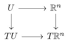
The operative notion that underlies this result is conjugacy. Suppose that \(r\) denotes the flow on the chart parametrizing the invariant slow manifold. The flow and the integral curves on a parametrised invariant manifold are linked to those of the underlying chart via the functional relationship

\( D\phi \cdot r = F \circ \phi, \)

or equivalently, by a commuting diagram:

Conjugacy is the basis of the parametrization method. The naive idea is to formally expand the reduced vector field

\( r(\xi,\epsilon) = \epsilon r_1(\xi) + \epsilon^2 r_2(\xi) + \cdots \)

and a smooth embedding

\( \phi(\xi,\epsilon) = \phi_0(\xi) + \epsilon \phi_1(\xi) + \epsilon^2 \phi_2(\xi) + \cdots \)

of the slow manifold in powers of \(\epsilon\), and to match terms in the conjugacy equation. We arrive at a list of so-called infinitesimal conjugacy equations for \(i = 1,2,\cdots\), of the form

\( \mathcal{F}(r_i,\phi_i) = G_i(\phi_0,\cdots,\phi_{i-1},r_1, \cdots, r_{i-1}). \)

So far the iteration is implicit: we need to solve the above equation for \((r_i,\phi_i)\) in terms of the quantities \(\phi_0,\cdots,\phi_{i-1},r_1, \cdots, r_{i-1}\) by `inverting \(\mathcal{F}\).' The operator \(\mathcal{F}\) is not invertible; under reasonable geometric conditions, however, the operator is surjective, and all of the infinitesimal conjugacy equations can be solved. The nonuniqueness of solutions for \((r_i,\phi_i)\) is related to the nonunique representation of \(S_{\epsilon}\), depending on which embedding is chosen. More explicit forms of the iteration can be obtained through the use of projectors.

A very similar procedure is applied to obtain approximations of the fast fiber bundle. The flow on the fast fiber bundle is conjugate to the flow of a normally nondegenerate bundle on the chart, and analogous infinitesimal conjugacy equations are obtained for the fibers.

It is interesting to highlight the `conservation of difficulty' in concocting this method, compared to the CSP method. In the CSP method, the iteration is explicitly defined, but showing that the \(i\)th iterate of the method provides the corresponding \(i\)th order approximation to the slow manifolds and fast fibers (equivalently, identifying the correct near-identity transformations in the iterations) requires a tedious amount of analysis. In the parametrization method, starting from the conjugacy assures that the \(i\)th order terms are the appropriate terms in the asymptotic expansion; on the other hand, knowing whether the infinitesimal conjugacy equations can all be solved is not obvious and requires proof. We also point out that approximations to the flow on the slow manifold as well as the dynamics on the fiber bundle are simultaneously calculated in the parametrization method, but not in the CSP method.

2.1. Probing multiple timescales

The conjugacy diagram in the previous section is easily extended to handle multiple-timescale problems:

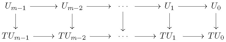
Geometrically, this corresponds to a nesting of invariant manifolds, each supporting a flow on a distinguished timescale (see Figure 2). The implication is that at each level of the nesting, we encounter another singular perturbation problem.

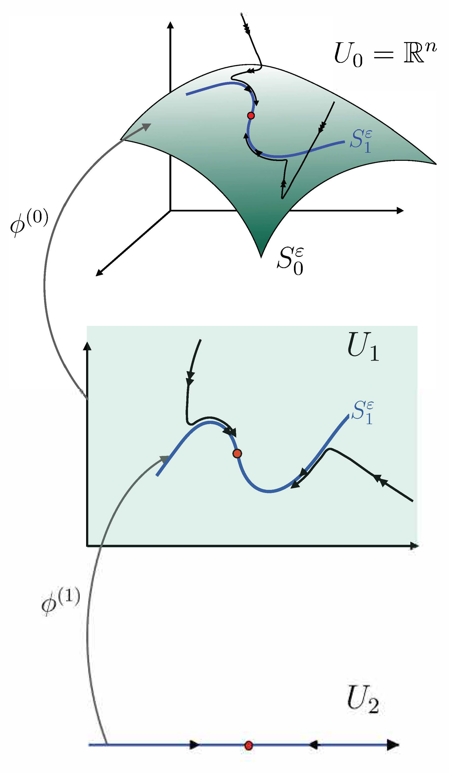
Figure 2. Sketch of a multiple timescale dynamical system having two nested slow invariant manifolds \(S_0^{\epsilon}\) and \(S_1^{\epsilon}\). The coordinate chart \(U_1\) is embedded as \(S_0^{\epsilon}\subset U_0 = \mathbb{R}^n\) by \(\phi^{(0)}\), and the coordinate chart \(U_2\) is embedded as \(S_1^{\epsilon}\subset U_1\) by \(\phi^{(1)}\). The red point depicts the possibility of a lower-dimensional invariant object (e.g. an equilibrium point, or a further submanifold introducing yet another dynamical timescale).

The parametrization method reveals some surprises in the world of multiple-timescale systems. A GSPT researcher might encounter a problem like

\( z' = H_0(z) + \epsilon H_1(z) \)

(2.2)

and expect two dynamical timescales; in fact, extra timescales may be hidden inside lower-dimensional invariant submanifolds, and these hidden timescales may dominate the long-term behavior of typical trajectories.

Consider the following system which models a hypothetical incoherent feed-forward loop (IFFL) an important motif in biochemical networks:

\( \begin{pmatrix} x_1' \\ x_2' \\ x_3' \end{pmatrix} = \begin{pmatrix} 0 \\ 0 \\ -x_3 \end{pmatrix} + \epsilon \begin{pmatrix} a_1 x_3 - a_2 x_1 x_2 \\ a_3 x_3 - a_4 x_2 \\ 1 \end{pmatrix}, \)

where \(0 < \epsilon \ll 1\) and \(a_i = \mathcal{O}(1)\) (i.e. the decay rate of the species \(x_3\) is much larger than all the other reaction rates). Note that this system is given in the standard form (0.2). This system admits a two-dimensional attracting invariant manifold \(\{x_3 = \epsilon\}\). Rescaling time as \(t_1 = \epsilon t\), we identify another two-timescale problem on this manifold, given by

\( \begin{pmatrix} \frac{dx_1}{dt_1} \\ \frac{dx_2}{dt_1} \end{pmatrix} = \begin{pmatrix} -a_2 x_1 x_2 \\ -a_4 x_2\end{pmatrix} + \epsilon \begin{pmatrix} a_1 \\ a_3 \end{pmatrix}. \)

(2.3)

Note that this reduced system is given in the more general form (0.1) (specifically, of the form (2.2). A further one-dimensional invariant submanifold \(\{x_2 = \epsilon a_3/a_4, x_3 = \epsilon\}\) is easy enough to calculate. The flow on this curve (on the infra-slow timescale \(t_2 = \epsilon^2 t\)) is governed by

\( \frac{dx_1}{dt_2} = a_1 - \frac{a_2 a_3}{a_4} x_1. \)

(2.4)

The parametrization method demystifies the emergence of such hidden timescales in more complicated problems. The term \( G_2\) in the second infinitesimal conjugation consists of several terms, only one of which is the coefficient of an \(\epsilon^2\) term in the vector field; in other words, derivatives of \(\phi_0,\phi_1,H_0,H_1\) can conspire to produce nontrivial \(\mathcal{O}(\epsilon^2)\) flow on a lower-dimensional submanifold. Note that these derivatives are related to intrinsic geometric characteristics of the dynamical system, like the curvature of the vector field and the invariant manifolds. In the IFFL example, the geometric `culprit' giving rise to infra-slow flow turns out to be a term depending on \(DH_1\) and \(\phi_1\) (the \(\epsilon\)-order term in the embedding \(\phi = \phi_0 + \epsilon \phi_1 + \cdots\) of \(S_{\epsilon}\)).

References

[1]   P. Cardin and M. Teixeira, Fenichel Theory for Multiple Time Scale Singular Perturbation Problems, SIADS, 16 (2017), pp. 1425-1452.

[2]   E. Feliu, N. Kruff, and S. Walcher, Tikhonov-Fenichel reduction for parametrized critical manifolds with applications to chemical reaction networks, J. Nonlinear Sci., 2020.

[3]   N. Fenichel, Geometric singular perturbation theory for ordinary differential equations, J. Differential Equations, 31 (1979), pp. 53-98.

[4]   A. Goeke and S. Walcher, A constructive approach to quasi-steady state reduction, J. Math. Chem., 52 (2014), pp. 2596-2626.

[5]   R. Heinrich and M. Schauer, Quasi-steady-state approximation in the mathematical modeling of biochemical networks, Math. Biosci., 65 (1983), pp. 155-170.

[6]   A. Zagaris, H. G. Kaper, and T. J. Kaper, Analysis of the Computational Singular Perturbation Reduction Method for Chemical Kinetics, J. Nonlinsci., 14 (2004), pp. 59-91.

[7]   A. Zagaris, H. G. Kaper, and T. J. Kaper, Fast and Slow Dynamics for the Computational Singular Perturbation Method, Multiscale Model. Simul., 2 (2004), pp. 613-638.

[8]   H. G. Kaper, T. J. Kaper, and A. Zagaris, Geometry of the Computational Singular Perturbation Method, Math. Model. Nat. Phenom., 10 (2015), pp. 16-30.

[9]   I. Kosiuk and P. Szmolyan, Geometric analysis of the Goldbeter minimal model for the embryonic cell cycle, J. Math. Biol., 72 (2016), pp. 1337-1368.

[10]   N. Kruff and S. Walcher, Coordinate-independent singular perturbation reduction for systems with three time scales, Math Biosci. Eng., 16 (5), pp. 5062-5091.

[11]   C. Kuehn, Multiple Time Scale Dynamics, Springer International Publishing Switzerland, 2015.

[12]   S. H. Lam and D. A. Goussis, The CSP Method for Simplifying Kinetics, Int. J. Chem. Kinetics, 26 (1994), pp. 461-486.

[13]   S. H. Lam and D. A. Goussis, Understanding complex chemical kinetics with computational singular perturbation, Symposium (International) on Combustion, 22 (1989), pp. 931-941.

[14]   I. Lizarraga and M. Wechselberger, Computational singular perturbation method for nonstandard slow-fast systems, SIAM J. Appl. Dyn. Sys., 19 (2020), pp. 994-1028.

[15]   I. Lizarraga, B. Rink, and M. Wechselberger, Multiple timescales and the parametrisation method in geometric singular perturbation theory, Preprint (2020), arXiv:2009.10583.

[16]   K. D. Mease, Geometry of Computational Singular Perturbations, IFAC Proceedings Volumes, 28 (1995), pp. 855-861.

[17]   M. Valorani, D. Goussis, F. Creta, and H. Najm, Higher order corrections in the approximation of low-dimensional manifolds and the construction of simplified problems with the CSP method, J. Comp. Phys., 209 (2005), pp. 754-786.

[18]   M. Wechselberger, Geometric singular perturbation theory beyond the standard form, Springer International Publishing, 2020.