Sean Gasiorek, University of Sydney ([email protected]).

1. Introduction

Mathematical billiards is a dynamical system consisting of a connected set \(\Omega\) (the billiard table) and a point-mass in its interior (the billiard ball) which moves in a straight line at constant speed. When the ball hits the boundary the ball reflects elastically and follows the rule of geometric optics: "angle of incidence equals angle of reflection." See [11, 28] for a thorough examination of billiards.

In magnetic billiards, the billiard ball is seen as a particle of charge \(e\) under the influence of a magnetic field B. The motion is determined by the Lorentz force, and upon collision with the boundary the billiard is governed by the same reflection principle. Billiards (both magnetic and otherwise) can be studied geodesic flow on a Riemannian manifold with (or without) boundary, and for the purposes of this article we will restrict the discussion to planar billiards in \(\mathbb{R}^{2}\) with the Euclidean metric.

Within the last decade there has been a small revival of the subject of integrability in magnetic billiards. Section 2 outlines the relevant properties of Birkhoff billiards that can be studied in the magnetic setting. Sections 3 and 4 address fundamental properties of magnetic and inverse magnetic billiards, and integrability in those magnetic variants of Birkhoff billiards.

2. Birkhoff Billiards

2.1. Introduction and Examples

Birkhoff considered billiards as a fundamental example of a dynamical system in the 1920's [9]. Let \(\Omega \subset \mathbb{R}^{2}\) be a strictly convex domain with smooth boundary \(\partial\Omega\) of length \(L\). Parametrize \(\partial \Omega = \Gamma\) by arc length \(s\). At a collision point of the billiard with the boundary, the point \(p_i = \Gamma(s_i)\), measure the angle \(\theta_i\) as the angle between the inward velocity vector immediately following the collision and the positive tangent (with respect to the induced orientation of \(\partial \Omega\)) at \(p_i\). Identifying \(\partial\Omega\) with \(\mathbb{R}/L\mathbb{Z}\), the billiard map is

\(T_1: \mathbb{R}/L\mathbb{Z} \times (0,\pi) \longrightarrow \mathbb{R}/L\mathbb{Z} \times (0,\pi), \qquad (s_i,\theta_i) \mapsto (s_{i+1},\theta_{i+1}) \)

and has the following properties:

a) If \(\partial \Omega = \Gamma\) is of class \(C^r\) then \(T_1\) is \(C^{r-1}(\mathbb{R}/L\mathbb{Z} \times (0,\pi))\)
b) \(T_1\) can be extended continuously to the boundary of its domain \(T_1(\cdot,0) = T_1(\cdot,\pi) = Id\)
c) \(T_1\) is symplectic; it preserves the area form \(d\omega = \sin(\theta)d\theta \wedge ds\)
d) \(T_1\) is a twist map
e) \(T_1\) has a generating function (unique up to an additive constant)

\(h(s_i,s_{i+1}) := - \| \Gamma(s_{i+1})-\Gamma(s_i)\| \)

where \(\| \cdot\|\) is the Euclidean distance. In particular, this means that \(\frac{\partial h}{\partial s_i} = \cos(\theta_i)\) and \(\frac{\partial h}{\partial s_{i+1}} = -\cos(\theta_{i+1}).\)

Example 1 (Billiards in a Circle). Suppose \(\Omega\) is a circle of radius \(R>0\). The map can be written explicitly as \(T_1(s,\theta) = (s+2R\theta,\theta)\) and the angle \(\theta\) is an integral of motion. Another integral of motion is the expression \(yu-xv\) for reflection point \((x,y)\) and inward velocity vector \((u,v)\).

If \(\theta\) is \(\pi\)-rational, the orbit is periodic. For every fully reduced \(p/q \in (0,1/2]\) there exist infinitely many periodic orbits with rotation number \(p/q\). And for each \(p/q \in (0,1/2]\), there is a time-reversed orbit which traces out the same periodic trajectory in reverse, and this reversed trajectory has rotation number \(1-p/q = (q-p)/q \in [1/2,1)\). A billiard with this property has time reversal symmetry.

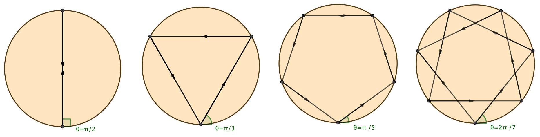
Figure 1. Periodic orbits of billiards in a circle with rotation numbers 1/2, 1/3, 1/5, and 2/7, respectively. The time-reversed orbits have rotation numbers 1/2, 2/3, 4/5, and 5/7, respectively.

If \(\theta\) is not \(\pi\)-rational, the trajectory will intersect the boundary in a dense set of points and will always remain tangent to a concentric circle of radius \(r = R|\cos(\theta)|\) after each reflection. This is an example of a convex caustic.

2.2. Caustics and Integrability

Definition 2. A convex caustic is a closed \(C^1\) curve in the interior of \(\Omega\), bounding itself a strictly convex domain, with the property that each trajectory that is tangent to it stays tangent after each reflection.

To a convex caustic in \(\Omega\) there is an invariant circle of \(T_1\) in phase space. The converse is not necessarily true: invariant circles give rise to caustics but are not necessarily convex or differentiable.

There are several ways to define integrability for Hamiltonian systems. The three on which we focus is Liouville-Arnol'd integrability (existence of integrals of motion), algebraic integrability (existence of polynomials in momenta/velocities on fixed energy levels), and \(C^0\)-integrability (existence of a foliation by invariant Lagrangian submanifolds). In the context of billiards, we can geometrically interpret \(C^0\)-integrability by showing that (part of) the billiard table is foliated by caustics. The previous example demonstrates that billiards in a circle are integrable in all three formulations.

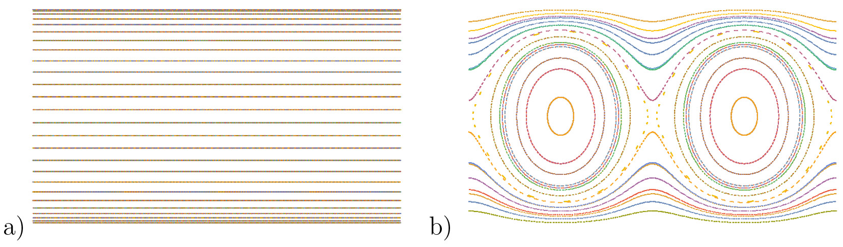
Figure 2. Phase space of the billiard in a circle (a) and ellipse (b).

A next natural question to ask relates to the existence or nonexistence of caustics in billiards.

• Do there exist examples of billiards with at least one caustic?
  Yes, by means of the string construction: Fix a convex caustic \(\gamma\) of length \(\ell\) and consider a closed, non-stretchable string of length strictly greater than \(\ell\). Pulling the string taut around \(\gamma\) to a point, move this point around \(\gamma\) and the resulting curve \(\Gamma\) will have \(\gamma\) as a caustic.
• Do there exist examples of billiards with infinitely many caustics?
  Yes, Lazutkin [21] proved that via a coordinate change every Birkhoff billiard is nearly integrable using a KAM-type theorem: a Cantor set of caustics accumulate near the boundary.
• Do there exist examples of billiards with no caustics?
  Yes, if the curvature of the boundary vanishes then no caustics can accumulate near the boundary [22]. This is a reason for assuming strict convexity of the billiard table \(\Omega\).
• Are there other billiards admitting a foliation by caustics?

Example 3 (Billiards in an Ellipse). Fix positive constants \(a \geq b>0\) and consider the billiard inside the ellipse with semi-major axis \(a\) and semi-minor axis \(b\). For every \(p/q \in (0,1/2)\), there exist infinitely many periodic orbits with rotation number \(p/q\), and exactly two period 2 orbits corresponding to the major and minor axes. Denote the foci of \(\Omega\) as \(\mathcal{F}_1,\mathcal{F}_2\). Any trajectory which crosses the segment \({\mathcal{F}_1\mathcal{F}_2}\) will also cross this segment upon reflection with the boundary; any trajectory which does not cross the segment \(\mathcal{F}_1\mathcal{F}_2\) will never cross \(\mathcal{F}_1\mathcal{F}_2\) after reflection with the boundary; and any trajectory which intersects one focus will subsequently intersect the other focus after reflection with the boundary. The first two cases correspond to trajectories with confocal hyperbolae and ellipses as caustics.

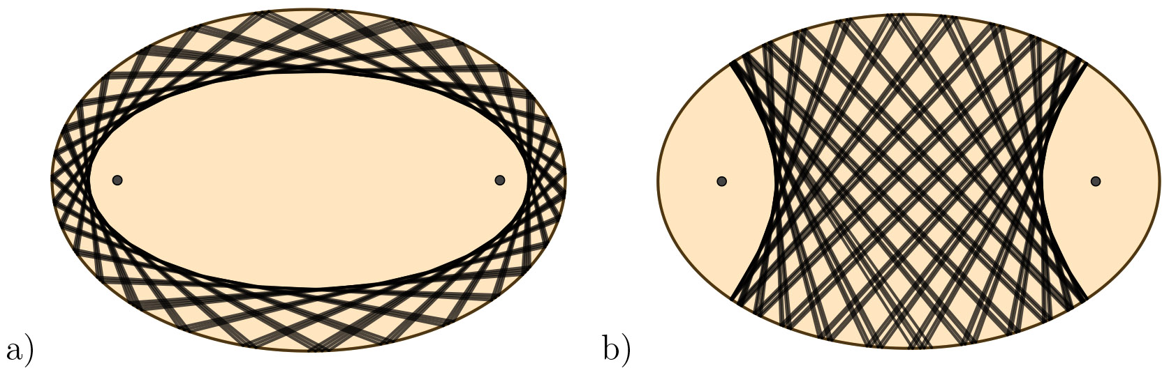
Figure 3. Billiards in an ellipse with a confocal ellipse (a) and hyperbola (b) as a caustic.

The elliptical table \(\Omega\) (with the exception of the segment \(\mathcal{F}_1\mathcal{F}_2\)) is foliated by convex caustics, and hence is \(C^0\)-integrable. In addition, \(\Omega\) is algebraically integrable (and hence Liouville-Arnol'd integrable): the function \(b^2xu + a^2yv\) is constant along trajectories with reflection point \((x,y)\) and velocity \((u,v)\).

Aside from the ellipse and circle, are there other examples of billiards that are \(C^0\)-integrable?

Conjecture 4 (Birkhoff). If the billiard inside \(\Omega\) is \(C^0\)-integrable, then \(\Omega\) is an ellipse.

The above conjecture was first explicitly formulated in [24] by Poritsky, student of Birkhoff, so the conjecture is sometimes referred to as the Birkhoff-Poritsky conjecture. Much work has been dedicated to proving this conjecture and its variants: In [6, 33], it is shown that the only billiards whose phase cylinder is foliated by rotationally-invariant curves are circles; in [2, 17], is it shown that if there exists a sequence of convex caustics with rotation numbers tending to one half, then the billiard is an ellipse; and in [18], a local version of the Birkhoff conjecture in a neighborhood of an ellipse is proved. When considering algebraic integrability, one can consider the algebraic Birkhoff conjecture:

Conjecture 5. If the billiard inside \(\Omega\) is algebraically integrable, then \(\Omega\) is an ellipse.

This has only recently been proven by Glutsyuk [14] for the plane and surfaces of constant curvature \(\pm 1\), provided that \(\partial \Omega = \Gamma\) is at least \(C^2\). At least the algebraic Birkhoff conjecture is now a theorem.

3. Magnetic Billiards

3.1. Introduction and Examples

Magnetic billiards was first studied in the mid 1980's [25, 26] and examined extensively over the last few decades [3, 7, 15, 30, 31]. Recently magnetic billiards has been studied in terms of Finsler billiards, where the magnetic flow is defined by a Finsler metric [16, 29]. We take a simplified approach. Consider a constant, homogeneous magnetic field B \(= (0,0,B)\) orthogonal to the billiard table and assume the billiard ball is a charged particle of charge \(e\). When in motion the particle moves under the influence of the Lorentz force, \(m\dot{v} = e(v \times\) B\()\), where \(\times\) is the cross product in \(\mathbb{R}^3\) and \(\cdot\) is the derivative with respect to time. The resulting dynamics is now uniform circular motion of Larmor radius \(\mu = m|v|/|eB|\), and we assume \(eB<0\) resulting in counterclockwise motion. As before, the billiard reflection law applies and the billiard within \(\Omega\) will consist of circular arcs of radius \(\mu\).

The dynamics is also dependent upon \(\mu\) in a nontrivial way. Robnik and Berry [25] described three curvature regimes based upon \(\rho\), the radius of curvature of \(\partial\Omega\):

\(\mu < \rho_{min}, \qquad \rho_{min}< \mu < \rho_{max}, \qquad \rho_{max}< \mu. \)

As before, we have a magnetic billiard map

\(T_2: \mathbb{R}/L\mathbb{Z} \times (0,\pi) \longrightarrow \mathbb{R}/L\mathbb{Z} \times (0,\pi), \qquad (s_i,\theta_i) \mapsto (s_{i+1},\theta_{i+1}) \)

and the properties (a–c) of the billiard map \(T_1\) are also true in this setting. However, only in the case \(\rho_{max}<\mu\) will \(T_2\) be a twist map. When twist, the map \(T_2\) will have rational rotation numbers \(p/q \in (0,1)\) because there is no time-reversal symmetry (a characteristic effect of magnetism). And when twist, the generating function is \(h(s_i,s_{i+1}) = -\ell - \frac{1}{\mu} \mathcal{S}\), where \(\ell\) is the length of the Larmor arc and \(\mathcal{S}\) is the area inside \(\Omega\) but outside the Larmor arc.

If \(\Omega\) is strictly convex, then any Larmor circle of radius \(\mu < \rho_{min}\) or \(\rho_{max}< \mu\) that is not tangent to \(\partial\Omega\) will only intersect the boundary in exactly two points, so successive collision points are well-defined. In the intermediate curvature regime, it is possible for a trajectory to become tangent to \(\partial \Omega = \Gamma\) from the inside, causing discontinuities in the map \(T_2\) due to these tangencies.

Example 6 (Magnetic Billiards in a Circle). If \(\Omega\) is a circle of radius \(R>0\), the extreme radii of curvature are equal to \(R\), so there are only two curvature regimes to consider. The magnetic billiard map can be written explicitly as \(T_2(s,\theta) = (s+2R\psi,\theta)\) where \(\psi\) is the angle between the inward velocity vector and the chord connecting successive collision points. Again, the angle \(\theta\) is an integral of motion, as is the angle \(\psi\). In particular, \(\psi = \psi(R,\mu,\theta)\) and can be computed explicitly using the geometry of circle-circle intersection. One can also state an integral of motion as the distance between the center of the Larmor circles and the center of the circular billiard table: \(x^2 + y^2 + 2\mu(uy-vx)\) is constant for reflection point \((x,y)\) and inward velocity vector \((u,v)\).

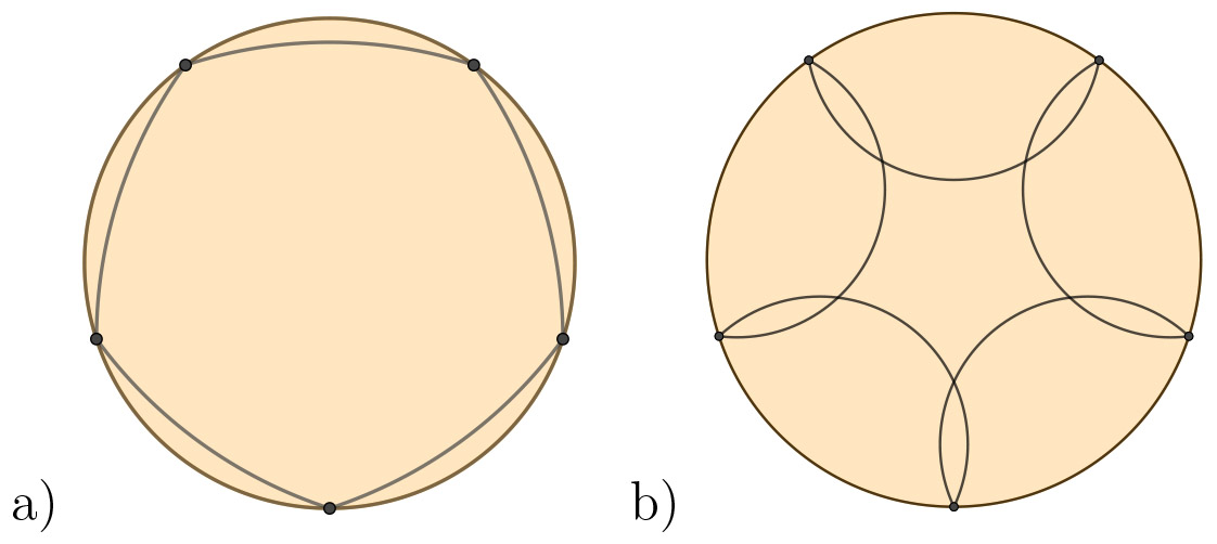
Figure 4. Circular magnetic billiards with period 5 and (a) rotation number 1/5 with \(\mu > \rho_{max} = R\); (b) rotation number 4/5 with \(\mu < \rho_{min} = R\).

Example 7 (Magnetic Billiards in an Ellipse). In the ellipse \(x^2/a^2 + y^2/b^2=1\) with \(a>b>0\), a direct calculation yields \(\rho_{min} = b^2/a\) and \(\rho_{max}= a^2/b\). The magnetic billiard in each curvature regime can be markedly different, which can be seen in the half-phase portraits in figure 5. Each curvature regime has regions of phase space foliated by invariant curves near \(\theta = \pi\), which correspond to short skips backwards along the boundary.

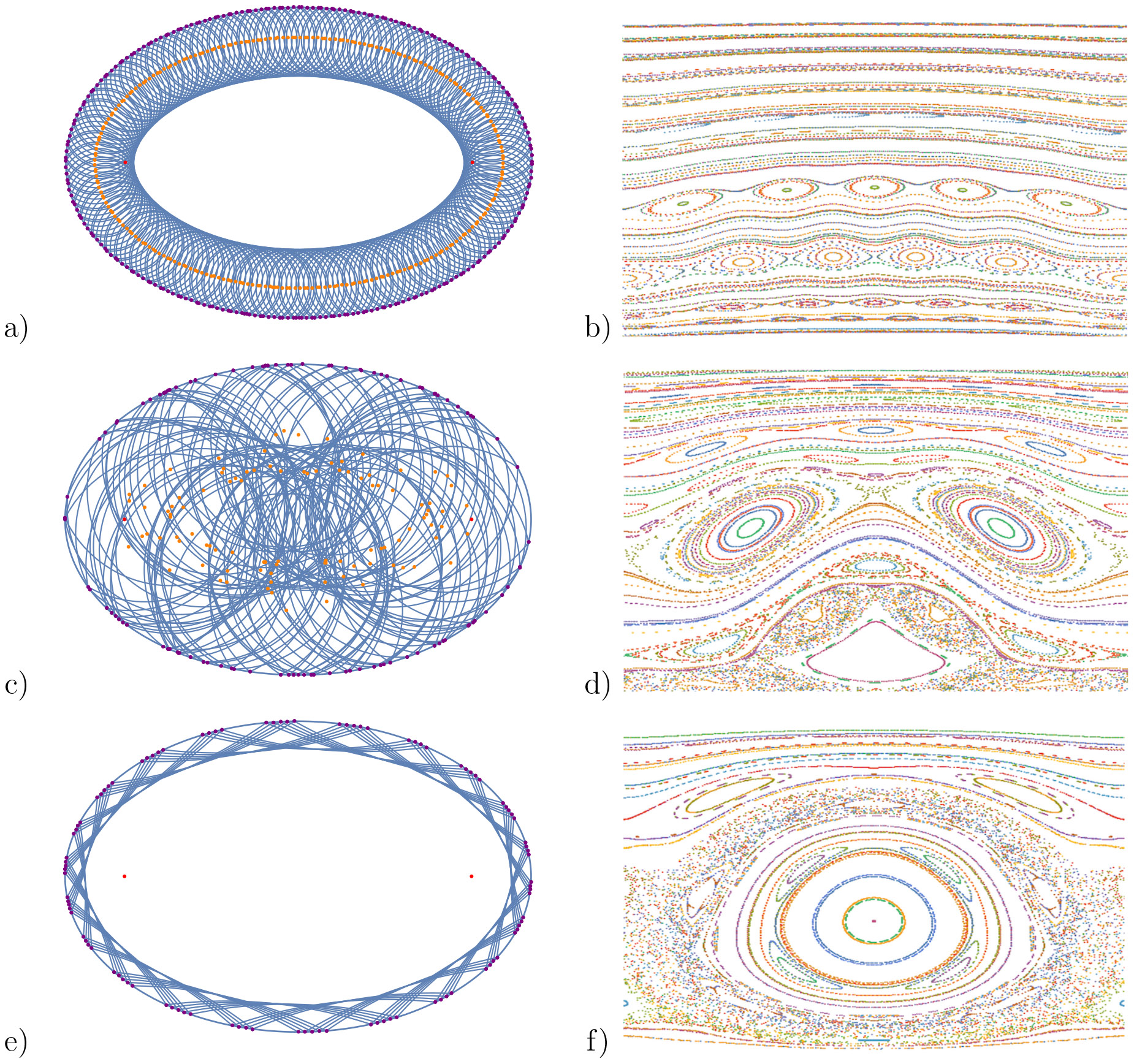
Figure 5. Magnetic billiard trajectories and half of phase space for \(\mu < \rho_{min}\) (a) and (b), \(\rho_{min} < \mu < \rho_{max}\) (c) and (d), and \(\rho_{max}<\mu\) (e) and (f).

3.2. Caustics and Integrability

As seen the examples above and in more detailed numerical simulations of an ellipse [1], magnetic billiards in strictly convex billiard tables shows a mix of near-integrable and chaotic behavior, depending upon the curvature regime and the relative size of \(\mu\). We again can ask about the (non)existence of caustics.

• Do there exist examples of billiards with at least one caustic?
  Yes, by means of an analogous string construction. Fixing the caustic, the level sets of a particular function form the billiard table with the given caustic [16, 29].
• Do there exist examples of billiards with infinitely many caustics?
  Yes, Berglund and Kunz [3] prove that a positive-measure set of caustics accumulate near the boundary in three cases, provided \(\partial \Omega = \Gamma\) is at least \(C^6\): \(\theta\) near 0 and \(\mu < \rho_{min}\); \(\theta\) near 0 and \(\rho_{max}<\mu\); or \(\theta\) near \(\pi\) for all values of \(\mu\).
• Do there exist examples of billiards with no caustics?
  This is unclear. The theorem of Berglund and Kunz above shows that caustics can still persist even if the table is non-convex (i.e., curvature \(\kappa <0\) but still sufficiently small), so the condition is not the same as for Birkhoff billiards.

Again, we can ask if there are other magnetic billiards admitting a foliation by caustics.

Conjecture 8. If the magnetic billiard inside \(\Omega\) is \(C^0\)-integrable, then \(\Omega\) is a circle.

The work of Bialy [7] proves that in the case of \(\mu < \rho_{min}\), if the billiard is \(C^0\)-integrable, then \(\Omega\) is a circle. Recent work by Bialy, Mironov, and others addresses the algebraic integrability of magnetic billiards. In particular, the work of [4, 5] prove that, for magnetic billiards in the plane and on surfaces of constant positive and negative curvature in the regime \(\rho_{max}< \mu\), if a polynomial integral in the velocities exists, then \(\Omega\) must be a circle. A similar result is proved in [8] for the regime \(\mu < \rho_{min}\).

4. Inverse Magnetic Billiards

4.1. Introduction and Examples

First introduced by [32] and studied further by others [10, 19, 20, 23, 27] in the context of semiconductors and condensed-matter physics and by the author [12, 13], inverse magnetic billiards is a combination of Birkhoff billiards and magnetic billiards in the following way: Define a magnetic field B that is 0 inside \(\Omega\) and constant magnitude \(B\) orthogonal to the plane outside \(\Omega\), and interpret the billiard table \(\Omega\) as a permeable boundary between magnetic and non-magnetic regions in the plane. The trajectories of a charged particle billiard are now straight lines inside \(\Omega\) concatenated with circular arcs of fixed Larmor radius \(\mu\) outside \(\Omega\). As in the case of magnetic billiards, we assume the motion outside \(\Omega\) is in the counterclockwise direction.

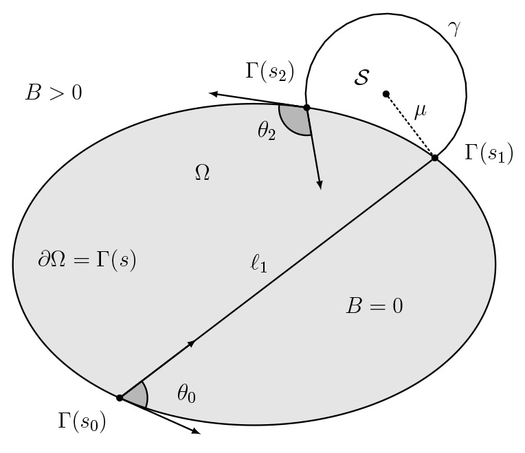
Figure 6. A labeled picture of the inverse magnetic billiard map \(T_3\).

We can define the inverse magnetic billiard map as the composition

\(\widehat{T_2} \circ T_1 := T_3: \mathbb{R}/L\mathbb{Z} \times (0,\pi) \to \mathbb{R}/L\mathbb{Z} \times (0,\pi), \qquad (s_i, \theta_i) \mapsto (s_{i+2},\theta_{i+2}), \)

where we interpret \(\widehat{T_2}\) as the magnetic billiard map corresponding to motion outside \(\Omega\). The map \(T_3\) possesses the same properties as \(T_2\), namely properties (a–c) of the map \(T_1\). The map \(T_3\) is a twist map in the case \(\mu < \rho_{min}\), and in such a case has rational rotation numbers \(p/q \in (0,1)\) and generating function \(h(s_i,s_{i+2}) = -\ell_1 - \gamma + \frac{1}{\mu}\mathcal{S}\), where \(\ell_1\) is the length of the chord inside \(\Omega\), \(\gamma\) is the length of the Larmor arc outside \(\Omega\) and \(\mathcal{S}\) is the area inside the Larmor arc but outside \(\Omega\), see figure 6. As in the case of magnetic billiards, we can consider the same three curvature regimes based on the relative sizes of the minimum and maximum radii of curvature of \(\partial\Omega\) and \(\mu\).

Just as in the case of magnetic billiards, if \(\Omega\) is strictly convex and \(\mu < \rho_{min}\) or \(\rho_{max}<\mu\), then the Larmor arcs will intersect \(\partial\Omega\) in exactly two places – the exit and reentry points of \(\Omega\). In the intermediate curvature regime, it is possible for the Larmor arc to become tangent to \(\partial\Omega\), leading to discontinuities in the map \(T_3\).

With inverse magnetic billiards, the strength of the magnetic field is fixed at the outset, which in turn fixes \(\mu\). But if we consider a single trajectory like figure 6, we can consider the two extremes in \(B\). As \(B \to \infty\), \(\mu \to 0\) and so \(T_3 \to T_1\), the Birkhoff billiard map; and as \(B \to 0^+\), \(\mu \to \infty\) and so \(T_3 \to Id\), the identity map. This statement can be made more rigorous, but it informs what we might expect from phase portraits in the two extreme curvature regimes.

Example 9 (Inverse Magnetic Billiards in a Circle). If \(\Omega\) is a circle of radius \(R\), the map can be written explicitly as \(T_3(s,\theta) = (s+2R\chi,\theta)\), where \(\chi\) is the angle between the outward velocity vector and the chord connecting exit and reentry points. Again, the angles \(\theta\), \(\chi\) are integrals of motion. In particular, \(\chi = \chi(R,\mu,\theta)\) and can be computed explicitly using the geometry of circle-circle intersection, and plays a similar role to \(\psi\) in example 6. As in the case of magnetic billiards, another integral of motion is the distance between the centers of the magnetic arcs and the table.

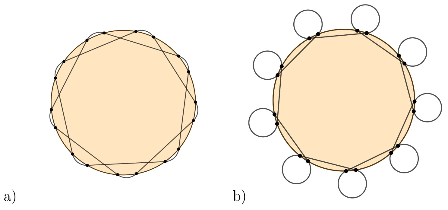
Figure 7. Inverse magnetic billiards in a circle with rotation numbers 2/9 (a) and 8/9 (b).

Example 10 (Inverse Magnetic Billiards in an Ellipse). In the ellipse \(x^2/a^2 + y^2/b^2=1\) with \(a>b>0\), again \(\rho_{min} = b^2/a\) and \(\rho_{max}= a^2/b\). The inverse magnetic billiard in each curvature regime can be markedly different, which can be seen in the half-phase portraits in figure 8. Each curvature regime has regions of phase space foliated by invariant curves near \(\theta = \pi\), which correspond to short billiard segments backwards along the boundary followed by a long circular arc outside \(\Omega\), reentering near the exit point.

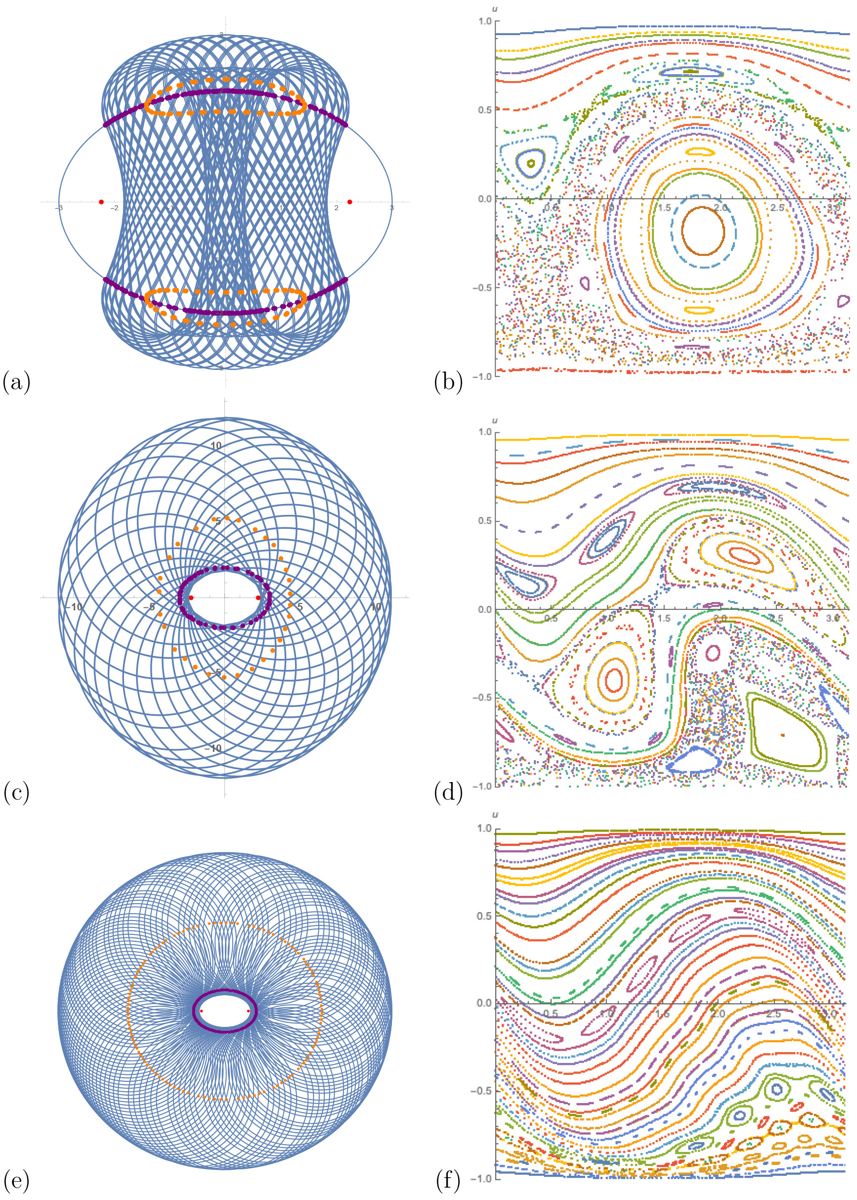
Figure 8. Trajectories with interior and exterior caustics and half of phase space for \(\mu < \rho_{min}\) (a) and (b), \(\rho_{min} < \mu < \rho_{max}\) (c) and (d), and \(\rho_{max}<\mu\) (e) and (f).

4.2. Caustics and Integrability

The phase portraits in figure 8 show similarities to figure 5, indicating the influence of the magnetic field in the dynamics of inverse magnetic billiards. Trajectories now extend outside \(\Omega\), and so there is now the notion of interior and exterior caustics, as can be seen in figure 8. In the case of the circle, there will be a concentric circular interior caustic of radius \(r_{interior} = R|\cos(\theta)|\) and an exterior concentric circular caustic of radius \(r_{outer} = \mu + \sqrt{\mu^2 + R^2 - 2R\mu\cos(\theta)}\). We can again ask about the (non)existence of caustics.

• Do there exist examples of billiards with at least one caustic?
  It is unknown if there is an analogous string construction for interior or exterior caustics.
• Do there exist examples of billiards with infinitely many caustics?
  Yes. Using a similar approach to the magnetic billiards case, in [12, 13] it is proved that a positive-measure set of interior caustics accumulate near the boundary in three cases, provided \(\partial \Omega = \Gamma\) is at least \(C^6\): \(\theta\) near 0 and \(\mu < \rho_{min}\); \(\theta\) near 0 and \(\rho_{max}<\mu\); or \(\theta\) near \(\pi\) for all values of \(\mu\).
• Do there exist examples of billiards with no caustics?
  If \(\partial\Omega\) has a point of vanishing curvature, there can be no interior caustics, similar to Birkhoff billiards. This is unknown in the case of exterior caustics.

At this time little is known about interior or exterior caustics beyond the above statements. It is unknown if the existence of an interior caustic implies the existence of an exterior caustic, or vice-versa. In the cases when \(T_3\) is not a twist map, caustics can exist though they may be \(C^0\) curves, as seen in the figure below.

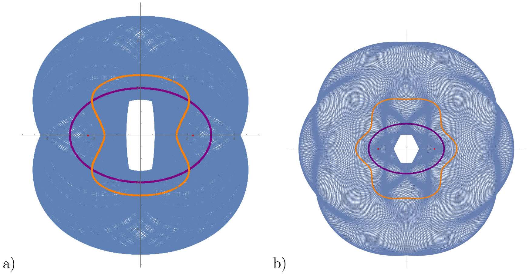
Figure 9. Inverse magnetic billiards in an ellipse with (a) \(\rho_{min}<\mu < \rho_{max}\) and (b) \(\rho_{max}< \mu\) showing \(C^0\) interior and exterior caustics. The Larmor centers are also shown to lie on a continuous curve.

Similar to the case of magnetic billiards, we can state a Birkhoff conjecture for integrability of inverse magnetic billiards:

Conjecture 11. If the inverse magnetic billiard on \(\Omega\) is \(C^0\)-integrable, then \(\Omega\) is a circle. If the inverse magnetic billiard on \(\Omega\) is algebraically integrable, then \(\Omega\) is a circle.

Acknowledgements

This material is based upon work supported by the National Science Foundation under Grant # DMS-1440140 while the author was in residence at the Mathematical Sciences Research Institute in Berkeley, California, during the Fall 2018 semester. This work was also supported by Discovery Project # DP190101838, Billiards within confocal quadrics and beyond from the Australian Research Council.

References

[1]   P. Albers, G. D. Banhatti, and M. Herrmann, Numerical simulations of magnetic billiards in a convex domain in \(\mathbb{R}^2\), 2017, https://arxiv.org/abs/1702.06309.

[2]   M. Arnold and M. Bialy, Non-smooth convex caustics for birkhoff billiard, Pacific Journal of Mathematics, 295 (2017), pp. 257–269, https://doi.org/10.2140/pjm.2018.295.257.

[3]   N. Berglund and H. Kunz, Integrability and ergodicity of classical billiards in a magnetic field, Journal of Statistical Physics, 83 (1996), pp. 81–126, https://doi.org/10.1007/BF02183641.

[4]   P. Albers, G. D. Banhatti, and M. Herrmann, Convex billiards and a theorem by E. Hopf, Mathematische Zeitschrift, 214 (1993), pp. 147–154, https://doi.org/10.1007/BF02572397.

[5]   M. Bialy, On totally integrable magnetic billiards on constant curvature surface, Electronic Research Announcements, 19 (2012), p. 112, https://doi.org/10.3934/era.2012.19.112.

[6]   M. Bialy and A. E. Mironov, Algebraic non-integrability of magnetic billiards, Journal of Physics A: Mathematical and Theoretical, 49 (2016), p. 455101, https://doi.org/10.1088/1751-8113/49/45/455101.

[7]   M. Bialy and A. E. Mironov, Polynomial non-integrability of magnetic billiards on the sphere and the hyperbolic plane, Russian Mathematical Surveys, 74 (2019), pp. 187–209, https://doi.org/10.1070/rm9871.

[8]   M. Bialy, A. E. Mironov, and L. Shalom, Magnetic billiards: Non-integrability for strong magnetic field; Gutkin type examples, Journal of Geometry and Physics, 154 (2020), p. 103716, https://doi.org/10.1016/j.geomphys.2020.103716.

[9]   G. Birkhoff, Dynamical Systems, American Mathematical Society, Providence, RI, 1927.

[10]   G. Casati and T. Prosen, Time Irreversible Billiards with Piecewise-Straight Trajectories, Phys. Rev. Lett., 109 (2012), p. 174101, https://doi.org/10.1103/PhysRevLett.109.174101.

[11]   N. Chernov and R. Markarian, Chaotic Billiards, American Mathematical Soc., 2006.

[12]   S. Gasiorek, On the Dynamics of Inverse Magnetic Billiards, PhD thesis, University of California Santa Cruz, 2019.

[13]   S. Gasiorek, On the dynamics of inverse magnetic billiards, 2019, https://arxiv.org/abs/1911.08144.

[14]   A. Glutsyuk, On polynomially integrable birkhoff billiards on surfaces of constant curvature, 2017, https://arxiv.org/abs/1706.04030.

[15]   B. Gutkin, Hyperbolic Magnetic Billiards on Surfaces of Constant Curvature, Communications in Mathematical Physics, 217 (2001), pp. 33–53, https://doi.org/10.1007/s002200000346.

[16]   E. Gutkin and S. Tabachnikov, Billiards in Finsler and Minkowski geometries, Journal of Geometry and Physics, 40 (2002), pp. 277–301, https://doi.org/10.1016/S0393-0440(01)00039-0.

[17]   N. Innami, Geometry Of Geodesics For Convex Billiards And Circular Billiards, Nihonkai Math. J., 13 (2002), pp. 73–120.

[18]   V. Kaloshin and A. Sorrentino, On the local Birkhoff conjecture for convex billiards, Annals of Mathematics, 188 (2018), pp. 315–380, https://doi.org/10.4007/annals.2018.188.1.6.

[19]   B. Kocsis, G. Palla, and J. Cserti, Quantum and semiclassical study of magnetic quantum dots, Physical Review B, 71 (2005), p. 075331, https://doi.org/10.1103/PhysRevB.71.075331.

[20]   A. Kormáanyos, P. Rakyta, L. Oroszláany, and J. Cserti, Bound states in inhomogeneous magnetic field in graphene: Semiclassical approach, Phys. Rev. B, 78 (2008), p. 045430, https://doi.org/10.1103/PhysRevB.78.045430.

[21]   V. F. Lazutkin, The Existence of Caustics for a Billiard Problem in a Convex Domain, Mathematics of the USSR-Izvestiya, 7 (1973), pp. 185–214, https://doi.org/10.1070/IM1973v007n01ABEH001932.

[22]   J. N. Mather, Glancing billiards, Ergodic Theory and Dynamical Systems, 2 (1982), pp. 397–403, https://doi.org/10.1017/S0143385700001681.

[23]   A. Nogaret, Electron dynamics in inhomogeneous magnetic fields, Journal of Physics: Condensed Matter, 22 (2010), p. 253201, https://doi.org/10.1088/0953-8984/22/25/253201.

[24]   H. Poritsky, The billard ball problem on a table with a convex boundary – an illustrative dynamical problem, Annals of Mathematics, 51 (1950), pp. 446–470, http://www.jstor.org/stable/1969334.

[25]   M. Robnik, Regular and chaotic billiard dynamics in magnetic fields, Nonlinear Phenomena and Chaos, 1 (1986), pp. 303–330.

[26]   M. Robnik and M. V. Berry, Classical billiards in magnetic fields, J. Phys. A: Math. Gen., 18 (1985), pp. 1361–1378, https://doi.org/10.1088/0305-4470/18/9/019.

[27]   H.-S. Sim, G. Ihm, N. Kim, and S. J. Lee, Magnetic Edge States in a Magnetic Quantum Dot, Physical Review Letters, 80 (1998), p. 4.

[28]   S. Tabachnikov, Remarks on magnetic flows and magnetic billiards, Finsler metrics and a magnetic analog of Hilbert's fourth problem, in Modern Dynamical Systems and Applications, 2004, pp. 233–250, http://arxiv.org/abs/math/0302288.

[29]   S. Tabachnikov and Pennsylvania State University Mathematics Advanced Study Semesters, Geometry and Billiards, Student mathematical library, American Mathematical Society, 2005.

[30]   T. Tasnádi, Hard Chaos in Magnetic Billiards (On the Euclidean Plane), Communications in Mathematical Physics, 187 (1997), pp. 597–621, https://doi.org/10.1007/s002200050151.

[31]   T. Tasnádi, The behavior of nearby trajectories in magnetic billiards, Journal of Mathematical Physics, 37 (1996), pp. 5577–5598, https://doi.org/10.1063/1.531723.

[32]   Z. Vörös, T. Tasnádi, J. Cserti, and P. Pollner, Tunable Lyapunov exponent in inverse magnetic billiards, Physical Review E, 67 (2003), p. 065202, https://doi.org/10.1103/PhysRevE.67.065202.

[33]   M. P. Wojtkowski, Two applications of Jacobi fields to the billiard ball problem, Journal of Differential Geometry, 40 (1994), pp. 155–164, https://doi.org/10.4310/jdg/1214455290.