1. Introduction: stability of traveling waves

The subject of this article is the stability of traveling pulses in reaction-diffusion equations

\( u_t=Du_{xx}+f(u) \),

(1.1)

where \(x\in\mathbb R\), \(u\in\mathbb R^n\), and \(D>0\) is diagonal. Specifically, we will discuss intrinsic criteria for stability–that is, features of a wave (or its ambient phase space) that explain why it is stable or unstable. Such criteria are important for two reasons. First, proving that a wave is (un)stable entails finding eigenvalues of a differential operator, which is generally a hard task. Using information from a wave's construction to assess its stability can make that task considerably easier. Second, by relating stability to wave properties, we gain a much deeper understanding of what drives a structure to be stable or unstable. Since stable structures tend to be the ones that we observe in nature, intrinsic criteria for stability are critical for understanding things like natural pattern formation.

Our goal herein is to explain how and why wave features relate to the eigenvalue equation that determines stability. From there, we will briefly introduce the tools that capture the relevant wave features. We will then close by specializing to the case of singularly perturbed systems, which are particularly suitable to analysis by these techniques. As an example, we will introduce a new mechanism for destabilizing fast traveling waves in the FitzHugh-Nagumo system. We begin with a few definitions and a statement of the eigenvalue problem.

A traveling pulse is a solution \(\hat{u}\) to (1.1) of one variable \(z=x-ct\), which travels in one direction with fixed profile and speed \(c\). To be a pulse, we also require that \(\hat{u}(z)\) decays exponentially as \(z\rightarrow\pm\infty\) to a constant value \(u_\infty\). Writing (1.1) in a moving frame, we see that a traveling pulse \(\hat{u}(z)\) is a fixed point (i.e., a time-independent solution) for the evolution equation

\( u_t=Du_{zz}+cu_z+f(u) \).

(1.2)

The definition of (asymptotic) stability matches our intuition from finite-dimensional dynamical systems: if \(u(z,t)\) is another solution to (1.2) whose initial profile is close to \(\hat{u}(z)\), then its profile must approach that of \(\hat{u}\) as \(t\rightarrow\infty\). Likewise, the strategy for proving stability emulates the finite-dimensional case. One typically begins by proving spectral stability, which is to say that the spectrum of the linearization of (1.2) about \(\hat{u}\) is contained in the left half-plane. The next step is to prove that spectral stability implies nonlinear stability (via linear stability). Although this latter step is more complicated for PDEs, it is generally understood how to achieve this, e.g. [16].

We therefore focus our attention on the eigenvalue equation

\( \lambda P = DP_{zz}+cP_z+f'(\hat{u}(z))P:=LP \).

(1.3)

In particular, the goal is to find all values \(\lambda\in\bar{H}^+:=\{z\in\mathbb C:\Re z\geq0 \}\) such that (1.3) has a bounded solution \(P:\mathbb R\rightarrow\mathbb C^n\). To tackle this problem, we introduce \(Q=P_z\) to convert (1.3) to a first-order system

\( Y'(z)=\left(\begin{array}{c} P\\Q \end{array}\right)_z=\left(\begin{array}{c c} 0 & I\\ D^{-1}(\lambda-f'(\hat{u}(z))) & -cD^{-1} \end{array}\right)\left(\begin{array}{c} P\\Q \end{array}\right) := A(\lambda,z)Y(z) \).

(1.4)

Notice that there is a well-defined limit

\( A(\lambda)=\lim\limits_{z\rightarrow\pm\infty}A(\lambda,z) \),

(1.5)

which is also achieved exponentially quickly. Viewing (1.4) as a perturbation of the constant coefficient system \(Y'(z)=A(\lambda)Y(z)\), it stands to reason that the stable and unstable subspaces of \(A(\lambda)\) would play a prominent role in the dynamics of (1.4). This is indeed the case, provided that \(A(\lambda)\) has no eigenvalues of zero real part. For simplicity, we assume:

For all \(\lambda\in\bar{H}^+, A(\lambda)\) has exactly \(n\) eigenvalues each of positive and negative real part.

Under this assumption, one can show (e.g., [1, section 3]) that, for all \(\lambda\in\bar{H}^+\), there exist sets

\( E^s(\lambda,z) = \{Y(z)\in\mathbb C^{2n}:Y(z) \) solves (1.4) and \( Y(z)\rightarrow 0 \) as \( z\rightarrow\infty \} \) \( E^u(\lambda,z) = \{Y(z)\in\mathbb C^{2n}:Y(z) \) solves (1.4) and \( Y(z)\rightarrow 0 \) as \( z\rightarrow-\infty \}, \)

(1.6)

which contain all solutions to (1.4) that are bounded in forward and backward time respectively. These sets are called the stable and unstable bundles. One should think of them as the set of solutions of (1.4) satisfying the right and left boundary conditions respectively. Since (1.4) is linear, each of \(E^{u/s}(\lambda,z)\) is a vector space (of dimension \(n\)) for fixed \(\lambda,z\). The solutions are real if \(\lambda\in\mathbb R\). This allows us to restate the eigenvalue condition:

Definition 1. \(\lambda\in\bar{H}^+\) is an \(\textbf{eigenvalue}\) for (1.3) if and only if \(E^s(\lambda,z)\cap E^u(\lambda,z)\neq\{ 0\}\) for some (hence all) \(z\in\mathbb R\).

In principle, one could study (1.3) or (1.4) independently of (1.2). However, (1.4) is non-autonomous, and the generic exponential growth of solutions complicates numerical calculations. (Not to mention that there are uncountably many potential eigenvalues to check!) There is also something unsatisfying about focusing entirely on (1.3). Suppose that you show that \(\lambda=7\) is an eigenvalue, so \(\hat{u}\) is unstable. While that may solve this problem, it doesn't give any indication as to how to solve the next eigenvalue problem. More importantly, solving (1.3) for \(\lambda=7\) does not give any indication as to why \(\hat{u}\) is unstable.

Instead, our goal is to consider (1.2) and (1.3) jointly. To that end, we first observe that \(\hat{u}_z\) solves (1.3) with \(\lambda=0\):

\( 0=D\hat{u}_{zz}+c\hat{u}_z+f(\hat{u})\implies0=D\hat{u}_{zzz}+c\hat{u}_{zz}+f'(\hat{u}(z))\hat{u}_z(z)=L\hat{u}_z \)

(1.7)

Furthermore, \(\hat{u}_z\) satisfies the boundary conditions, so \(\lambda=0\) is an eigenvalue, and \((\hat{u}_z,\hat{u}_{zz})\in E^u(0,z)\cap E^s(0,z)\). We call \(\lambda=0\) the translation eigenvalue because it reflects the fact that \(\hat{u}(z+k)\) is also a traveling wave solution of (1.2) for any \(k\in\mathbb R\).

To take this a step further, we can write the traveling wave ODE as a first order system by setting \(u_t=0\) and \(u_z=v\) in (1.2):

\( \left(\begin{array}{c} u\\v \end{array}\right)_z=\left(\begin{array}{c} v\\-D^{-1}(cv+f(u)) \end{array}\right) \).

(1.8)

Written this way, the traveling pulse \(\varphi(z):=(\hat{u},\hat{u}_z)\) is a homoclinic orbit to the fixed point \(p:=(u_\infty,0)\in\mathbb R^{2n}\). By definition, this means that \(\varphi(z)\in W^u(p)\cap W^s(p)\) for all \(z\in\mathbb R\). Consequently, \(\varphi'(z)\), which we already know lies in the intersection \(E^u(0,z)\cap E^s(0,z)\), must be tangent to \(W^u(p)\) and \(W^s(p)\). It is easy to show that the following, stronger result is true.

Theorem 1.1. The unstable bundle \(E^u(0,z)\) is the tangent space \(T_{\varphi(z)}W^u(p)\) to the unstable manifold \(W^u(p)\) at each point \(\varphi(z)\). Likewise, \(E^s(0,z)=T_{\varphi(z)}W^s(p)\) all along \(\varphi\).

This theorem is one way of stating the fact that (1.4) is the equation of variations for (1.8) when \(\lambda=0\).

2. The Evans function and Maslov index: a crash course

There is a famous tool for finding eigenvalues, originally due to Evans [9, 10, 11, 12]. The stable and unstable bundles are each \(n\)-dimensional vector spaces (for fixed \(\lambda,z\)), and (1.4) is defined on \(\mathbb C^{2n}\). By taking bases for each space, one can therefore check for intersections (i.e., eigenvalues) by evaluating the Wronskian determinant

\( \det\left[E^s(\lambda,z),E^u(\lambda,z) \right] \).

(2.1)

If this determinant vanishes for some \(\lambda=\lambda_*\), then \(E^u(\lambda_*,z)\cap E^s(\lambda_*,z)\neq \{0\},\) hence \(\lambda_*\) is an eigenvalue. This determinant is essentially the Evans function. To make the definition rigorous, one can consider the equation induced on exterior powers of \(\mathbb C^{2n}\) by (1.4). For the details, we refer the reader to [1]. Although (2.1) appears to be \(z\)-dependent, this dependence can be removed easily by using Abel's formula. As result, one obtains a function \(D(\lambda)\)–the Evans function–which satisfies the following properties.

(1) \(D(\lambda)\) is analytic on a domain \(\mathcal{D}\) containing \(\bar{H}^+\), and \(D(\lambda)\in\mathbb R\) for all \(\lambda\in\mathbb R\cap\mathcal{D}\).
(2) Zeros of \(D\) correspond to eigenvalues in (1.3).
(3) The multiplicity of \(\lambda\) as a root of \(D\) equals the algebraic multiplicity of \(\lambda\) as an eigenvalue.

The value of the analyticity of \(D(\lambda)\) is that the argument principle can be used to count unstable eigenvalues. If \(K\) is a simple, closed loop containing all potentially unstable eigenvalues in its interior, then the winding number of \(D\) around \(K\) gives a count of eigenvalues inside \(K\), thus informing the stability of the traveling wave \(\hat{u}(z)\). This procedure does, however, involve varying \(\lambda\), so it is not directly tied to the traveling wave equation itself.

As is the case for fixed points of vector fields, only one unstable eigenvalue is needed to prove instability of a traveling wave \(\hat{u}\). The following argument is frequently used to prove the existence of at least one unstable eigenvalue. As observed earlier, \(\lambda=0\) is necessarily an eigenvalue. It follows that \(D(0)=0\) as well. Moreover, it is easy to show that \(D(\lambda)>0\) for real \(\lambda\gg0\). Therefore, if \(D'(0)<0\), then there must exist some \(\lambda>0\) for which \(D(\lambda)=0\).

The Evans function parity argument just described explains why the value \(\lambda=0\) is particularly important from the spectral theory perspective. Theorem 1.1 explains why it is important from the dynamical systems perspective as well. Because (1.4) with \(\lambda=0\) is the equation of variations for (1.8), it is possible to relate the sign of \(D'(0)\) to changes in invariant manifolds of (1.8) as parameters are varied. In the case of traveling waves, this parameter is most often the speed \(c\). Below we will discuss fast traveling waves in the FitzHugh-Nagumo model, which is the paradigmatic application of this idea.

We just saw that phase space geometry provides a binary piece of information that relates to wave stability. The next question is whether we can glean more information from the traveling wave equation. This leads us to the Maslov index. To introduce the Maslov index, we change perspective slightly and consider the unstable bundle \(E^u(0,z)\) as a curve in the Grassmannian \(\mbox{Gr}_n(\mathbb R^{2n})\) of \(n\)-dimensional subspaces of \(\mathbb R^{2n}\). This space is a manifold, so one can talk about the homotopy class of curves.\(^1\) Specifically, we would like to use the topology of \(\mbox{Gr}_n(\mathbb R^{2n})\) to get better estimates on the count or location of eigenvalues.

Unfortunately, \(\pi_1(\mbox{Gr}_n(\mathbb R^{2n}))=\mathbb Z/2\mathbb Z\) for \(n\geq 2\), so there is not any new information beyond the parity result that we already have from the Evans function, in general. However, there is a submanifold of \(\mbox{Gr}_n(\mathbb R^{2n})\) whose topology is more amenable to our analysis. This is the set of Lagrangian subspaces \(\Lambda(n)\), which are those subspaces that are their own symplectic complement for a fixed symplectic form \(\omega\) defined on \(\mathbb R^{2n}\). It happens that \(\pi_1(\Lambda(n))=\mathbb Z\), so it is possible to assign a winding number to curves in this space. This winding number is the Maslov index.

The problem is then to prove that \(\Lambda(n)\) is an invariant submanifold for the equation induced on \(\mbox{Gr}_n(\mathbb R^{2n})\) by (1.4). In order for this to be the case, (1.2) must be either a gradient or skew-gradient system, which to say that the nonlinearity \(f(u)\) is an invertible diagonal matrix times a gradient [5, 6].\(^2\) For such systems, the Maslov index measures the winding of the unstable bundle \(E^u(0,z)\) in the tangent bundle above the wave. Since the unstable bundle is everywhere tangent to the unstable manifold \(W^u(p)\), it can be thought of as the (signed) number of twists that \(W^u(p)\) makes as it evolves along \(\hat{u}\). One can show that this index either gives an exact count or a lower bound on the number of real, positive eigenvalues for (1.3). See [5, 6, 17] and references therein.

The application of the Maslov index in this context can be thought of as a generalization of Sturm-Liouville theory to systems. For (1.1) with \(n=1\), the latter says that eigenvalues are real and simple, hence enumerable as \(\lambda_0>\lambda_1>\dots\). Moreover, the eigenfunction corresponding to \(\lambda_j\) has exactly \(j\) zeros. Using the fact that \(\hat{u}_z\) is a \(0\)-eigenfunction, one can therefore detect how many eigenvalues lie to the right of \(0\) by counting zeros of \(\hat{u}_z\). Viewing \((\hat{u},\hat{u}_z)\) in the phase plane and using Theorem 1.1, it is clear that this is precisely the winding of the unstable bundle. The challenge in moving to systems is that there are other solutions in \(E^u(0,z)\), hence the winding is occurring in a higher-dimensional place, namely \(\Lambda(n)\).

3. Geometric Singular Perturbation Theory

The focus of this article so far has been relating phase space geometry to stability indices–\(\mathrm{sign}\,D'(0)\) and the Maslov index. We have not yet mentioned the issue of obtaining the needed information from phase space. Indeed, this task is not trivial. In both cases, we need to follow an invariant manifold as it evolves along a homoclinic orbit. One class of problems for which such information is obtainable is singularly perturbed equations. We can use Geometric Singular Perturbation Theory (GSPT) to get a very accurate picture of the relevant invariant manifold. There is a long history of applications of the Evans function in singularly perturbed equations. A general framework for calculating the Maslov index in singularly perturbed equations was established in [7]. See [8] for a recent application to a higher-dimensional system.

Rather than giving a general overview of GSPT, we will instead apply it to the FitzHugh-Nagumo (FHN) model, which is the example we discuss in further detail in the next section. For more background on theory, we refer the reader to [13, 18, 23]. Readers who are familiar with GSPT and the FHN model may skip to the next section. The traditional FitzHugh-Nagumo model is the following system of equations:

\( \begin{aligned} u_t & =u_{xx}+f(u)-w\\ w_t & = \varepsilon(u-\gamma w). \end{aligned} \)

(3.1)

The nonlinearity \(f\) is given by \(f(u)=u(1-u)(u-a)\), with \(0<a<1>0\) fixed. We assume that \(\gamma >0\) is small enough so that the only homogeneous fixed point of (3.1) is \((u,w)=(0,0)\). Finally, we assume \(0<\varepsilon\ll 1\), making (3.1) singularly perturbed. The reader will notice that (3.1) is not of the form (1.1) because there is no diffusion on the second variable. This simply reduces the dimension of phase space from \(4\) to \(3\) when we cast the traveling wave ODE as a first-order system: 

\( \left(\begin{array}{c} u\\v\\w \end{array}\right)_z=\left(\begin{array}{c} v\\-cv+w-f(u)\\-\frac{\varepsilon}{c}(u-\gamma w) \end{array}\right). \)

(3.2)

As for the stability problem, the Evans function theory is unchanged. We cannot, however, use the Maslov index when the dimension of phase space is odd. The Maslov index does apply if \(w\) is allowed to diffuse at the same rate as \(u\), cf. [6, 7].

Sending \(\varepsilon\rightarrow0\) in (3.2) turns \(w\) into a parameter. This results in a one-dimensional set of critical points (i.e., a center manifold):

\( M_0=\{(u,v,w):v=0,w=f(u)\}. \)

(3.3)

Away from these critical points, the dynamics of (3.2) with \(\varepsilon=0\) and \(\varepsilon>0\) will be similar. However, on or near \(M_0\)–where the vector field in (3.2) is \(O(\varepsilon)\)–the situation is more complicated. For example, only the point \(0:=(u,v,w)=(0,0,0)\) is a fixed point for \(\varepsilon>0\).

To see what happens in the vicinity of \(M_0\), we change timescales by setting \(\xi=\varepsilon z\) and denoting \(\dot{ }=\frac{d}{d\xi}\):

\( \left(\begin{array}{c} \varepsilon \dot{u}\\\varepsilon \dot{v}\\\dot{w} \end{array}\right)=\left(\begin{array}{c} v\\-cv+w-f(u)\\-\frac{1}{c}(u-\gamma w) \end{array}\right) \).

(3.4)

Sending \(\epsilon\rightarrow0\) in (3.4) yields a differential-algebraic equation where the flow is given by

\( \dot{w}=-\frac{1}{c}(u-\gamma w) \),

(3.5)

and it is restricted to the set \(M_0\). Formally, we therefore have the picture that the "fast" system (3.2) connects different points on \(M_0\), and then the "slow" system (3.4) takes over on \(M_0\). Shortly, we will construct a traveling pulse of (3.1) as a homoclinic orbit consisting of concatenated fast and slow segments.

Broadly speaking, the goal of GSPT is to reconcile the behavior of the fast and slow systems when \(\epsilon>0\). In our case, that amounts to showing that a singular homoclinic orbit consisting of four segments glued together persists when \(\epsilon\) is turned on. We now describe the singular orbit that forms the template of the traveling pulse.

The first segment is a "fast jump" in \(uv\)-space. Concretely, it is a heteroclinic orbit connecting \((u,v)=(0,0)\) to \((1,0)\). Such a connection exists only for speed

\( c=c^*:=\sqrt{2}(a-1/2)<0 \),

(3.6)

cf. [24]. The next segment is slow, occurring on \(M_0^R\)–the right branch of the cubic \(w=f(u)\) on which \(f'(u)<0\). Since \(c<0\), and \(u>\gamma w\) for \(u\) on \(M^R_0\), we see from (3.4) that the flow is in the direction of increasing \(w\). Eventually, we reach a point \((u^*,w^*)\) for which another heteroclinic orbit exists in the fast system. Using the symmetry of the cubic \(f\), one can show that this jump occurs at

\( (u^*,w^*)=((2/3)(a+1),f(u^*)) \).

(3.7)

Finally, there is a slow segment on \(M_0^L\)–the left branch of \(M_0\) on which \(f'(u)<0\)–that returns the pulse to the fixed point \(0\). A more detailed account of this construction can be found in many places, e.g. [21]. See Figure 1 for a picture of the singular orbit.

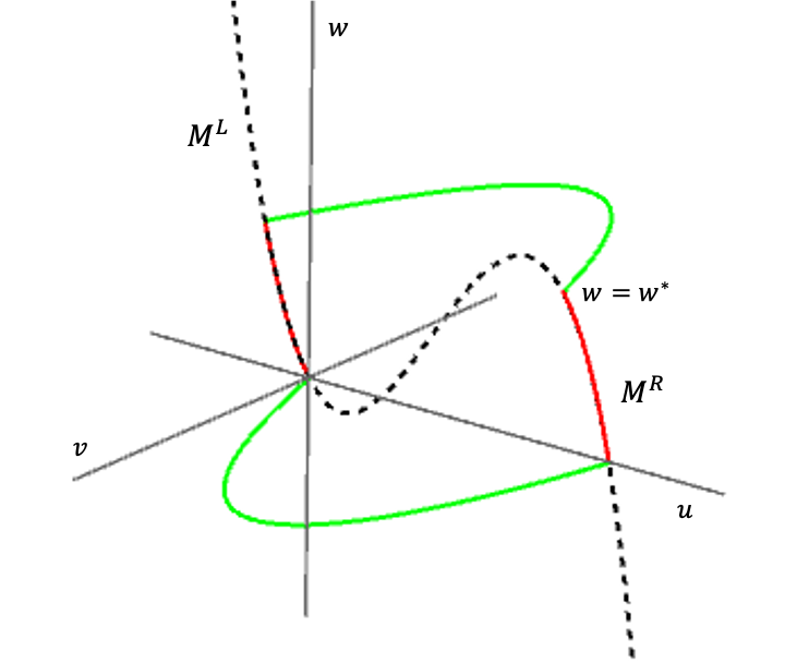
Figure 1. The singular orbit, which is \(O(\varepsilon)\) close to a traveling pulse solution of (3.1). In order, it consists of a (green) fast jump from the origin to \(u=1\), a (red) trip up the right slow manifold \(M^R\), a (green) fast jump back to \(M^L\) and a (red) return to the origin along \(M^L\).

GSPT provides the geometric tools for showing that the singular orbit above perturbs to an \(\epsilon>0\) traveling pulse of (3.1). It does so by giving persistence results for invariant manifolds, which can be shown to intersect in such a way that yields a homoclinic orbit. It is worth describing those manifolds here because they are also used to calculate the Maslov index and Evans function \(D'(0)\).

Recall that \(M_0\) is the set of critical points for the fast subsystem (3.2) with \(\epsilon=0\). For fixed \(w\), each of these points has one-dimensional stable and unstable manifolds as long as \(f'(u)<0\). By taking the union over all points in \(M_0^L\) (resp. \(M_0^R\)), we can therefore define two-dimensional sets \(W^{u/s}(M_0^{L})\) (resp. \(W^{u/s}(M_0^{R})\)). GSPT is built on three theorems about these sets, due to Fenichel [13].

First, the critical manifolds \(M_0^{L/R}\) perturb to slow manifolds \(M_\epsilon^{L/R}\), which are locally invariant relative to (3.2). The flow on \(M^{L/R}_\epsilon\), to leading order in \(\epsilon\), is given by (3.4). Second, the manifolds \(W^{u/s}(M_0^{L/R})\) also perturb to locally invariant manifolds \(W^{u/s}(M_\epsilon^{L})\) for (3.2). Finally, the foliation of \(W^{u/s}(M_0^{L})\) by the stable and unstable manifolds of individual points in \(M_0\) persists when \(\epsilon>0\). In other words, given a point \(p\in M_\epsilon^{L/R}\), one can identify stable and unstable manifolds \(W^{u/s}(p)\) which are locally invariant and diffeomorphic to the corresponding manifolds when \(\epsilon=0\).

Since the orbit we seek is homoclinic to \(0\), one would expect it to be constructed as the intersection of \(W^u(0)\) and \(W^s(0)\). However, in order to use a perturbation argument for the existence of the wave with \(\epsilon>0\), we need the \(\epsilon=0\) intersection to be transverse. By a dimension count, this cannot happen. To remedy this, we append the equation \(c'=0\) to (3.2) and instead look for an intersection of \(W^{cu}(0)\) and \(W^{cs}(0)\). This argument is successful, but it requires a technical result called the Exchange Lemma [20]. The Exchange Lemma addresses the problem of what happens to \(W^{cu}(0)\) as it passes near the right slow manifold \(M_\epsilon^R\). We mention this here because the information obtained from the Exchange Lemma is the exact ingredient used to prove that the fast traveling pulses are stable.\(^3\)

4. Destabilization of the FitzHugh-Nagumo fast traveling waves

In this section, we apply the insights gained from previous Evans function and Maslov index calculations to reveal a new mechanism for destabilizing fast traveling waves in the FitzHugh-Nagumo system. Before doing so, we give a brief summary of the stability result for the FHN fast traveling waves, due to Jones [19] and subsequently Yanagida [26]. The first step is to show that there are only two potentially unstable eigenvalues, each of which is \(O(\epsilon)\)-close to \(0\).\(^4\) Since we know that \(\lambda=0\) must be an eigenvalue, it follows that the other eigenvalue near \(0\) is real. The Evans function parity argument from section 2 is used to show that the other eigenvalue is negative, hence the waves are spectrally (linearly, and nonlinearly) stable.

The interesting part of this proof for our purposes is the manner in which \(\mathrm{sign}\,D'(0)\) is determined. Using Theorem 1.1 (actually, a slight variation thereof) and the Exchange Lemma, it can be shown that stability of the wave hinges on the direction in which \(W^u(M_\epsilon^R)\) and \(W^s(M_\epsilon^L)\) cross along the second heteroclinic connection (the "fast back"). Analytically, this direction is determined by calculating the Melnikov integral

\( \int_{-\infty}^{\infty}e^{c^*z}v_b(z)\,dz<0 \),

(4.1)

where \(v_b(z)\) is the \(v\)-component of the fast back connecting \(M_0^R\) to \(M_0^L\) with \(\epsilon=0\) [21, 22]. (We know this integral is negative because \(v_b\) is the derivative of \(u_b\), which decreases monotonically along the back.) This type of result is exactly what we are after in this article; the stability of the wave is determined by an observable feature of phase space, namely the way that two invariant manifolds intersect.

We will now show how the traditional FHN model can be altered slightly to flip the sign of this Melnikov integral, thus forcing \(D'(0)<0\) and destabilizing the fast traveling pulse. We will do so by rewriting the reaction term in the \(u\) equation of (3.1) as \(\tilde{f}(u,w)\). Assuming that a heteroclinic connection exists for the same value \(w=w^*\), one can check that the Melnikov integral (4.1) becomes

\( M=-\int_{-\infty}^{\infty}e^{c^*z}\partial_w\tilde{f}(u,w)|_{(u,w^*)}v_b(z)\,dz \).

(4.2)

Some care is required to specify \(\tilde{f}\). Comparing with (3.2) and (3.3), we see that the new critical manifold is given by \(M_0=\{(u,v,w):v=0,\tilde{f}(u,w)=0 \}\). In particular, it is no longer a graph, which makes it considerably harder to understand and control the dynamics. For inspiration, we turn to the Maslov index calculation that was used to prove that fast traveling pulses for (3.1) are stable when \(w\) diffuses [7]. In that paper, we showed that one can obtain the necessary information about how \(W^u(M_\epsilon^R)\) and \(W^s(M_\epsilon^L)\) cross just by looking at the corner where the slow-to-fast transition occurs on \(M_0^R\). (See section 4.4.) In particular, the orientation can be flipped if the tangent line to \(M_0^R\) changes from negative to positive slope.

With this guidance, we proceed to study the model

\( \begin{aligned} u_t & =u_{xx}+f(u)-h(w)\\ w_t & = \varepsilon(u-\gamma w), \end{aligned} \)

(4.3)

with \(f\) and all parameters as above. The classic model has \(h(w)=w\), so in an effort to make this alteration as small as possible, we set

\( h(w)=w+\eta(w) \).

(4.4)

We want \(\eta\) to be localized near \(w=w^*\), since it is just the back that we wish to change. The equation for the critical manifold \(M_0\) becomes \(h(w)=f(u)\), so in order to have \(\displaystyle\frac{dw}{du}>0\), we need \(h'(w^*)<0\), since \(f'(u^*)<0\). We therefore set

\( \eta(w):=(w^*-w)(1+\delta)e^{-\beta (w^*-w)^2} \).

(4.5)

We take \(0<\delta\ll 1\) (but fixed), and \(\beta\gg 1\). As \(\beta\rightarrow\infty\), \(||\eta(w)||_\infty\rightarrow0\), so we can view \(h(w)\) as providing an arbitrarily small perturbation of the original FHN model.\(^5\) For simplicity, we will also write \(\eta(w)=0\) for \(w=0\) so that the end state of the wave stays fixed. Since \(\eta\) decays rapidly anyway, this could easily be made official by multiplying \(\eta\) by a bump function supported in a neighborhood of \(w^*\). See Figure 2 for a plot of \(\eta(w)\).

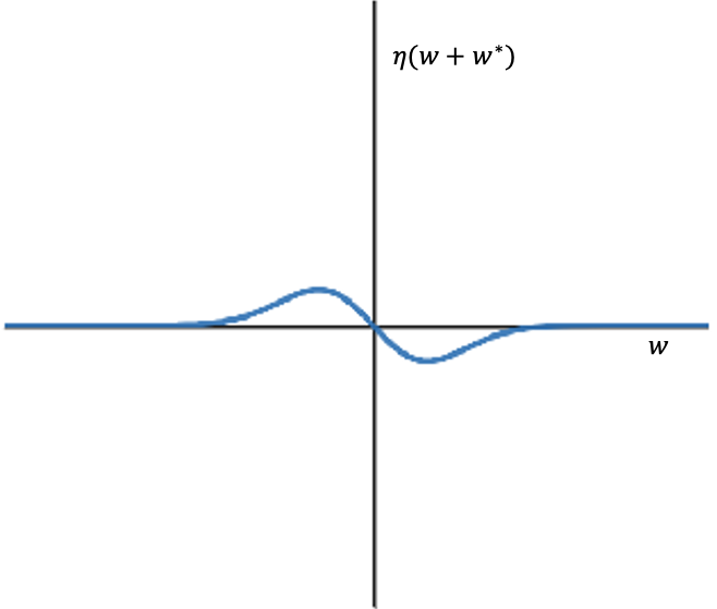
Figure 2. The perturbation \(\eta(w)\) applied to the \(u\) equation in the FitzHugh-Nagumo model (3.1). The origin is shifted to the jump-off point \(w^*\).

To see what effect this perturbation has on (4.3), we plot the nullclines with and without \(\eta\) in Figure 3. Near \(w=0\), the dynamics are completely unchanged. Thus we have a unique fast front (i.e., connection from \(M^L\) to \(M^R\)) for \(c=c^*\) and \(w=0\). For \(w=w^*\), the fast back exists as well, since \(h(w^*)=w^*\). However, since \(h\) is not monotone we have two additional solutions \(w_{\pm}\) to \(h(w)=w^*\) satisfying \(w_-<w^*<w_+\). This means that there are three distinguished singular orbits, all of which persist for \(\varepsilon>0\) as long as \(M\neq0\) in (4.2). From Figure 3b, we can see that the effect on the wave profile corresponding to \(w^*\) is to add a small tremor during the slow-fast transition.

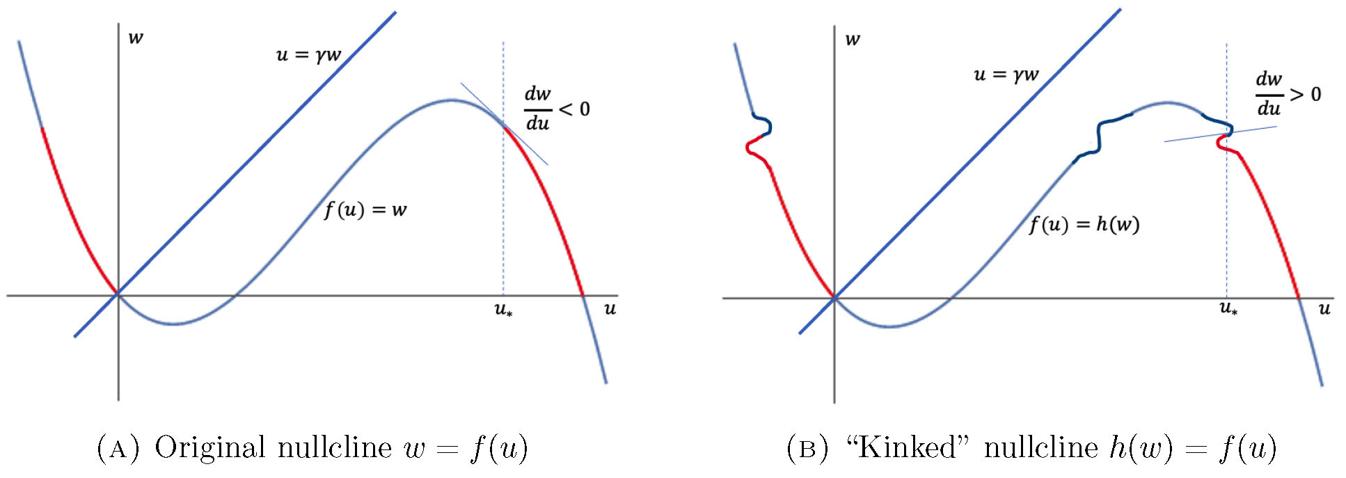
Figure 3. Picture of the slow flow and critical manifold in \(uw\)-space. The red segments of the curves are the slow orbits. By adding a "kink" to the nullcine through the \(\eta(w)\) perturbation, the slope of the tangent line to the curve \(h(w)=f(u)\) changes sign at the jump-off point \((u^*,w^*)\).

To prove that the \(\eta\) perturbation destabilizes the wave, we apply (4.2) to \(\tilde{f}(u,w)=f(u)-h(w)\):

\( M=\int_{-\infty}^{\infty}e^{c^*z}h'(w^*)v_b(z)\,dz \).

(4.6)

A straightforward computation gives that \(\eta'(w^*)=-(1+\delta)\), hence

\( h'(w^*)=1-(1+\delta)=-\delta<0 \).

(4.7)

Together, (4.6) and (4.7) imply that the wave exists (by the Exchange Lemma) and that it is unstable. A natural follow-up question is: what happens to time-dependent solutions of (4.3) whose initial profiles are close to this unstable wave? We can see from Figure 3b that \(h'(w_\pm)>0\). Thus the two extra traveling waves that are generated by this perturbation are both stable, by (4.6). Since \(w_-<w^*<w_+\), it is tempting to conjecture that the wave with \(\max(w(z))=w^*\) forms some kind of boundary between the basins of attraction for the stable waves. However, that exercise is left to the reader.

Remark 4.1. As mentioned earlier, the Maslov index can be used to study (3.1) when \(w\) diffuses and \(D=I\). In that case, the fast traveling wave is stable, just like its \(3\)D counterpart. Interestingly, the unstable waves constructed in this section cannot be studied with the Maslov index. This is because the nonlinearity in (4.3) needs to be skew-gradient, which means that a multiple of \(h'(w)\) would need to appear in the reaction term of the \(w\) equation. It turns out that the skew-gradient requirement forces an intersection of the nullclines on \(M_0^R\), which prevents the construction of the pulses.

\(^1\) \(E^u(0,z)\) is not actually a loop, but this detail can be smoothed over using the dual notions of intersection and winding numbers [2, 4, 25]. It is actually through intersections, and not winding, that the eigenvalue equation is related to the Maslov index. 

\(^2\) In recent work [3], we showed how a Maslov-type index can be defined for a dense subset of \(\mbox{Gr}_n(\mathbb R^{2n})\). This significantly broadens the class of systems that could be analyzed.

\(^3\) These pulses are called fast because the speed \(c\) is \(O(1)\) in \(\epsilon\). There are also slow traveling waves whose speed approaches \(0\) as \(\epsilon\rightarrow0\). The fast pulses are known to be stable, while the slow pulses are unstable [14].

\(^4\) This step actually brings another nice topological stability index into the mix. Starting with a Jordan curve \(K\) in the spectral plane as in section 2, one obtains a sphere by taking a product of \(K\) with the domain of the traveling pulse, which is \([-\infty,\infty]\). The unstable bundle \(E^u(\lambda,z)\) can then be viewed as a vector bundle over the sphere, and the count of eigenvalues inside \(K\) is equal to the first Chern number of this bundle [1]. This is particularly useful for singularly perturbed systems, because the unstable bundle decomposes into the Whitney sum of a fast and slow piece, and the Chern number is additive across such a sum. This idea matured into a fast-slow decomposition of the Evans function using the so-called "elephant trunk lemma" [15].

\(^5\) It is not, however, \(C^1\)-close since \(h'(w^*)=-\delta\) irrespective of \(\beta\), while \(\frac{d}{dw}w=1\). See (4.7).

References

[1]   J. Alexander, R. Gardner, and C. Jones, A topological invariant arising in the stability analysis of travelling waves, J. reine angew. Math, 410 (1990), p. 143.

[2]   V. I. Arnol'd, Characteristic class entering in quantization conditions, Functional Analysis and its applications, 1 (1967), pp. 1–13.

[3]   T. J. Baird, P. Cornwell, G. Cox, C. Jones, and R. Marangell, A Maslov index for non-Hamiltonian systems, arXiv preprint arXiv:2006.14517, 2020.

[4]   C.-N. Chen and X. Hu, Maslov index for homoclinic orbits of Hamiltonian systems, in Annales de l'Institut Henri Poincaré, vol. 24 of Analyse non Linéare, 2007, pp. 589–603.

[5]   C.-N. Chen and X. Hu, Stability analysis for standing pulse solutions to FitzHugh–Nagumo equations, Calculus of Variations and Partial Differential Equations, 49 (2014), pp. 827–845.

[6]   P. Cornwell, Opening the Maslov box for traveling waves in skew–gradient systems: counting eigenvalues and proving (in)stability, Indiana University Mathematics Journal, 68 (2019), pp. 1801–1832.

[7]   P. Cornwell and C. K. Jones, On the existence and stability of fast traveling waves in a doubly diffusive FitzHugh–Nagumo system, SIAM Journal on Applied Dynamical Systems, 17 (2018), pp. 754–787.

[8]   P. Cornwell, C. K. Jones, and C. Kiers, Bifurcation to instability through the lens of the Maslov index, arXiv preprint arXiv:2102.08852, 2021.

[9]   J. W. Evans, Nerve axon equations. i: Linear approximations, Indiana University Mathematics Journal, 21 (1972), pp. 877–885.

[10]   J. W. Evans, Nerve axon equations. ii: Stability at rest, Indiana University Mathematics Journal, 22 (1972), pp. 75–90.

[11]   J. W. Evans, Nerve axon equations. iii: Stability of the nerve impulse, Indiana University Mathematics Journal, 22 (1972), pp. 577–593.

[12]   J. W. Evans, Nerve axon equations. iv: The stable and the unstable impulse, Indiana University Mathematics Journal, 24 (1975), pp. 1169–1190.

[13]   N. Fenichel, Geometric singular perturbation theory for ordinary differential equations, Journal of Differential Equations, 31 (1979), pp. 53–98.

[14]   G. Flores, Stability analysis for the slow travelling pulse of the FitzHugh–Nagumo system, SIAM journal on mathematical analysis, 22 (1991), pp. 392–399.

[15]   R. Gardner and C. K. Jones, Stability of travelling wave solutions of diffusive predator-prey systems, Transactions of the American Mathematical Society, 327 (1991), pp. 465–524.

[16]   D. Henry, Geometric theory of semilinear parabolic equations, Lecture notes in mathematics, Springer-Verlag, Berlin, New York, 1981.

[17]   P. Howard, Y. Latushkin, and A. Sukhtayev, The Maslov and Morse indices for Schrödinger operators on \(\mathbb{R}\), Indiana University Mathematics Journal, 67 (2018).

[18]   C. Jones, Geometric singular perturbation theory, Dynamical systems, 1995, pp. 44–118.

[19]   C. Jones and N. Kopell, Tracking invariant manifolds with differential forms in singularly perturbed systems, Journal of Differential Equations, 108 (1994), pp. 64–88.

[20]   C. Jones, N. Kopell, and R. Langer, Construction of the FitzHugh–Nagumo pulse using differential forms, in Patterns and dynamics in reactive media, Springer, 1991, pp. 101–115.

[21]   C. K. Jones, Stability of the travelling wave solution of the FitzHugh–Nagumo system, Transactions of the American Mathematical Society, 286 (1984), pp. 431–469.

[22]   M. Krupa, B. Sandstede, and P. Szmolyan, Fast and slow waves in the FitzHugh–Nagumo equation, Journal of Differential Equations, 133 (1997), pp. 49–97.

[23]   C. Kuehn, Multiple time scale dynamics, vol. 191, Springer, 2015.

[24]   H. P. McKean, Nagumo's equation, Advances in mathematics, 4 (1970), pp. 209–223.

[25]   J. Robbin and D. Salamon, The Maslov index for paths, Topology, 32 (1993), pp. 827–844.

[26]   E. Yanagida, Stability of fast travelling pulse solutions of the FitzHugh–Nagumo equations, Journal of Mathematical Biology, 22 (1985), pp. 81–104.