Handling editor: Steve Schecter

Vasilis Dakos, Egbert van Nes, and Marten Scheffer,
Department of Aquatic Ecology and Water Quality Management Wageningen University, The Netherlands

What do ecosystems, neuron cells and financial markets have in common? They can all have tipping points at which sudden shifts to a different regime occur. In the jargon of complex systems, such shifts are considered to be critical transitions [MS1]. Such transitions are often very important for humans: fisheries that collapse threaten viable ecosystem services, neuron cells that fire in synchrony lead to epileptic seizures, financial markets that crash leave thousands of people unemployed.

Such critical transitions are ubiquous in a variety of complex systems; transitions in earth systems, ocean circulation patterns, the climate, human physiology, traffic jams, global finance are a few to mention. In all cases predicting the critical threshold at which the transition occurs is notoriously difficult, or considered impossible. Models are usually not accurate enough to provide reliable predictions. Thus it would be extremely useful to have empirical indicators that can tell us whether we are approaching a transition even in the absence of adequate knowledge about the mechanisms involved [MS2].

Indicators of upcoming transitions: theoretical expectations

It is well known that in complex systems a continuous change in a given parameter may sometimes lead to sudden changes in the behavior of the system through bifurcation points [RS] (figure 1a, b). Such bifurcations are usually associated with a vanishing dominant eigenvalue of the stable equilibrium (zero-eigenvalue bifurcations [SS], figure 1c, d). This implies that the system becomes increasingly slow in recovering from perturbations close to the critical point. Indeed, it can be shown that "critical slowing down" is a generic phenomenon in the particular class of first-order (i.e. discontinuous) and second-order (i.e. continuous) phase transitions and can be even found in other types of transitions (like the Hopf bifurcation from a stable point to a limit cycle).

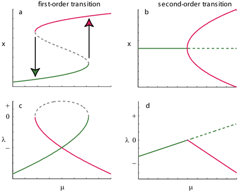
Figure 1. First-order discontinuous transition (a; fold bifurcation: x'=-x³+β x+μ) and second-order continuous transition (b; pitchfork bifurcation: x'= -x³+x μ). As the system approaches the bifurcation point the dominant eigenvalue λ of the system goes to zero: the fingerprint of "critical slowing down."

Direct consequences of critical slowing down are [MS2]:

• Slow recovery from perturbations: The recovery rate after small perturbations decreases when the system is close to the bifurcation (figure 2a, d).
• Increasing autocorrelation: The state of the system becomes more and more like its past state (figure 2c, f). The highly correlated time series close to the transition can be quantified as an increase in autocorrelation.
• Increasing variance: The accumulating impact of the non-decaying shocks prior to the transition increases the variance of the state variable (figure 2c, f).
• Increasing spatial coherence: Critical slowing down turns spatially coupled units less reactive close to the bifurcation. At this point diffusion between neighboring units dominates. As a result, units tend to be in a state similar to that of their neighbors. Such increasing coherence is measured as increased spatial correlation.

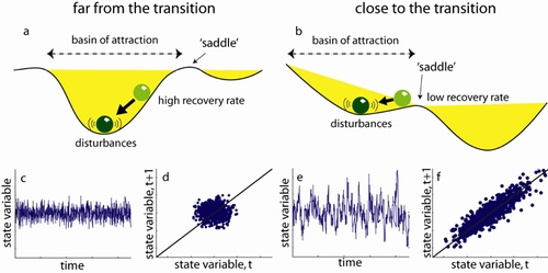
Figure 2. Characteristic changes in the dynamics of a system towards a first-order transition. a) Far from the transition a small perturbation is fast absorbed within the symmetric basin of attraction of the stable equilibrium. b) Close to the transition the system recovers slowly upon a perturbation. As a result variance (c, e) and autocorrelation (d, f) of the produced time series differ (modified from [MS2]).

Transitions are not though only associated with vanishing eigenvalues. They also are associated with multiple basins of attraction that a system jumps to. Such attraction basins are usually asymmetric close to the bifurcation, and are delimited by saddle points which topologically may be seen as hills on stability landscapes (figure 2a, d). Asymmetries and saddles can be also related to transition indicators:

• Increasing skewness: In the vicinity of saddles the rates of change are low (reflected in the asymmetry of the stability landscape; figure 2d). The system spends more time close to the saddle resulting in a highly skewed distribution of the state variable.
• Flickering: The probability that stochastic forcing may temporarily shift a system back and forth between alternative basins of attraction is higher close to a bifurcation. As a result, the variance and skewness of the frequency distribution of the state variable increases.
• Spatial patterns: In a wider class of spatial systems, precursors of critical transitions deviate from the above described general patterns. Instead they are associated with specific indicators, like self-organized pattern formation [MR], changing scale-invariant power-law structures [SK], and divergent order parameters [RS].

Can we monitor early-warning signals in real applications?

Most of the proposed leading indicators have been developed in simple models and have not yet been tested in the field. Despite the optimism that the few empirical successes inspire [e.g. VD], more work is needed to test their applicability. Apparently, for any leading indicator to be useful, some requirements are needed:

1. It needs to be easily measured.
2. It needs to be robust.
3. It needs to be identified early enough to allow timely action.

The biggest challenge in the application of early-warning signals comes from the difficulty in identifying the right variable to measure and the right scale for monitoring that variable. In theory the variable that will be the most reliable indicator would be the one representing the fast component of the system (the variable that actually shows that a transition has occurred; like the crashing biomass of a fisheries). However in practice some variables will be difficult or costly to measure at an adequate spatial or temporal resolution. Failing to correctly identify and adequately sample the right variables may lead to false negatives in recognizing upcoming transitions.

A positive trend in the proposed leading indicators in real data may not always be related to impending transitions. For instance a rare external event may trigger a shift (false negative). Or a trend in the external regime of perturbations may lead to false positives. The robustness of the indicators may be further challenged by the fact that there are multiple drivers that push the system not to a singularly defined transition point but towards a moving threshold. Perhaps tracking multiple indicators for multiple variables (and drivers) may be a promising solution in building robust indicator estimates.

All proposed early-warning signals are relative measures. They do not predict when a transition occurs, but only indicate that the likelihood of approaching a transition increases. This implies that it is difficult to assess when an indicator actually signifies that the fragility of the system is high that action is needed for averting a transition. Such task becomes even more difficult given the inertia of any system; intervention actions will only be successful if they are fast and able to exercise influence on the fast components of the system.

Looking forward

Early-warning signals are only indicative tools for recognizing impending shifts. Specific knowledge of the system dynamics, feedbacks and potential thresholds will always remain the most important components in understanding and managing any system. However the generic character of the early-warning signals provides optimism about our potential ability to forecast critical transitions.

References

[MR]		Rietkerk, M., S. C. Dekker, P. C. de Ruiter, and J. van de Koppel. 2004. Self-Organized Patchiness and Catastrophic Shifts in Ecosystems. Science 305:1926-1929.
[MS1]		Scheffer, M. 2009. Critical transitions in Nature and Society. Princeton University Press, Cambridge.
[MS2]		Scheffer, M., J. Bascompte, W. A. Brock, V. Brovkin, S. R. Carpenter, V. Dakos, H. Held et al. 2009. Early-warning signals for critical transitions. Nature 461:53-59.
[RS]		Solé, R.V., Manrubia, S.C., Luque, B., Delgado, J., and J. Bascompte. 1996. Phase transitions and complex systems. Complexity 1:13-26.
[SK]		Kefi, S., M. Rietkerk, C. L. Alados, Y. Pueyo, V. P. Papanastasis, A. ElAich, and P. C. de Ruiter. 2007. Spatial vegetation patterns and imminent desertification in Mediterranean arid ecosystems. Nature 449:213-217.
[SS]		Strogatz, S.H. 1994. Nonlinear Dynamics and Chaos with Applications to Physics, Biology, Chemistry and Engineering. Perseus Books.
[VD]		Dakos, V., Scheffer, M., van Nes, E.H., Brovkin, V., Petoukhov, V., Held, H. 2008. Slowing down as an early warning signal for abrupt climate change. Proc Natl Acad Sci U S A 105:14308-14312.