1. Introduction

The Nonlinear Schödinger Equation (NLS),

(1)

\( iq_t=q_{xx}\pm 2|q|^2q \),

is the prototypical example of a completely integrable nonlinear PDE, that is, one that can, to some degree, be solved explicitly [1]. Moreover, it arises from many different physical applications, from Bose-Einstein condensates to light traveling in optical fibers [2–8].

Many of these applications depend on understanding the dynamics and long-time behavior of highly disordered solutions. If we were studying a linear PDE, this task would be a simple one: we could assume the solutions were a linear combination of plane waves of the form \(e^{i(kx-\omega t)}\). The way the wave number \(k\) and frequency \(\omega\) of each plane wave are related, known as the dispersion relation, dictates how all solutions to that PDE will behave over time.

For example, for the linear Schrödinger equation describing a free particle, \(iq_t=q_{xx}\), substituting \(q\sim e^{-i(kx-\omega t)}\) yields the dispersion relation \(\omega=k^2\). From this, we can learn more about how waves travel: In this case, since \(\omega(k)\) is real-valued for \(k\) real, the modes evolve as harmonic waves. Since \(\omega''(k)\not\equiv0\), the evolution of these waves is dispersive in the sense that different plane waves travel with different velocities. The corresponding group velocity of wave packets centered at the wave number \(k\) is \(V_g=\omega'(k)=2k\) [9].

Since nonlinear waves generally need not evolve as harmonic superpositions of plane waves, the above linear picture does not apply. We can see, for example, that though the NLS has an exact plane wave solution

\( q(x,t) = A e^{i [k x + (k^2-2A^2)t]} \),

since its frequency \(\omega(k)=k^2-2A^2\) depends on the amplitude \(A\), one cannot obtain a dispersion relation that applies to all solutions. For nonlinear equations, we need a different approach.

When the nonlinear term is small, one can understand the long-time dynamics by using the dispersion relation from just the linear terms to derive an approximate solution to the nonlinear problem, which consists of weakly coupled, slowly modulated plane waves (with no nonlinear term, the plane waves would be completely decoupled). However, this approach shouldn't work if the small nonlinearity assumption is not valid (e.g. for the NLS, this would occur if the amplitude is large so \(|q|^2q\) is significant).

Interestingly, we find that many disordered solutions of the NLS with large amplitudes – situations where this assumption does not apply – still behave similarly to linear plane waves – on average, over long timescales [10]. Below, we will detail the methods that lead to this surprising result.

2. Nonlinear Dispersion Relation?

In more detail, the typical way of addressing the long-time dynamics of nonlinear equations is to assume the nonlinear term is small and use the dispersion relation from just the linear terms to derive an approximate solution to the nonlinear problem, which consists of weakly coupled, slowly modulated plane waves.

If we rescale the NLS with \(q \to q\alpha/\sqrt{2}\) to obtain \(iq_t=q_{xx}\pm \alpha^2 |q|^2q\), we can suppose \(\alpha\) is a small parameter and apply the method of multiple scales.

2.1. Multiple Scales Analysis

We first transform the NLS to wavenumber space by letting

(2)

\( q(x,t)=\sum_{n=-\infty}^{\infty}a_{k_n}(t)e^{-ik_n x} \),

with \(k_n=2\pi n/L\). We thus obtain the infinite set of ordinary differential equations

(3)

\( i\frac{d}{dt} a_{k_n} (t)= -k_n^2a_{k_n}(t)\pm \alpha^2\sum_{p,q,r=-\infty}^\infty a_{k_p}(t)a_{k_q}(t)a^*_{k_r}(t) \delta_{k_p+k_q-k_r-k_n,0} \)

for the wave modes \(a_{k_n}(t)\), where \(\delta_{j,l}\) is the Kronecker delta.

The solution of Eq. (3) assumes the form

\( a_{k_n}(t)= b_{k_n} (\tau) e^{i k_n^2 t} + O(\alpha^2) \),

where \(\tau=\alpha^2t\) is a slow variable, and \(b_{k_n} (\tau)\) satisfy the solvability condition

(4)

\( i\frac{d}{d\tau} b_{k_n}(\tau) = \pm \sum_{p,q,r=-\infty}^\infty b_{k_p}(\tau) b_{k_q} (\tau)b^*_{k_r}(\tau) e^{i(k_p^2+k_q^2-k_r^2-k_n^2)t} \delta_{k_p+k_q-k_r-k_n,0}\,\delta_{k_p^2+k_q^2-k_r^2-k_n^2,0} \).

It turns out that the equations

\( k_p+k_q-k_r-k_n = 0 \), \( k_p^2+k_q^2-k_r^2-k_n^2 = 0 \),

found in the delta functions, can only be solved if \(p=r\) and \(q=n\) or \(p=n\) and \(q=r\) [11]. Because of this, Eq. (4) simplifies significantly, and becomes

(5)

\( i\frac{d}{d\tau} b_{k_n}(\tau) =\pm \left(2 \sum_{m=- \infty}^\infty | b_{k_m} |^2 - | b_{k_n} |^2\right) b_{k_n}(\tau) \),

And in fact, because \(\sum |b_{k_m}|^2\approx\sum |a_{k_m}|^2= \| a_\kappa \|^2\) is the conserved total wave action, a little bit of manipulation will show that the terms in the parentheses are actually constant in \(\tau\). The solution to Eq. (5) is then

\( b_{k_n} = a_{k_n}(0) e^{\mp i \left(2 \| a_\kappa \|^2 - | a_{k_n} (0) |^2\right)\alpha^2 t} \),

and the NLS wave from Eq. (2) can be expanded as

(6)

\( q(x,t) = \sum_{n=-\infty}^{\infty}a_{k_n}(0) e^{-i\left[k_nx-\omega(k_n)t\right]} + O(\alpha^2) \),

where

(7)

\( \omega(k_n) \approx k_n^2 \mp \alpha^2 \left(2 \| a_\kappa\|^2 - |a_{k_n} (0) |^2\right) \).

This shows that the mode with the wavenumber \(k_n\) evolves in time with the effective frequency \(\omega(k_n)\).

If all the mode amplitudes in the EDR in Eq. (7) are small compared to the total wave action \(\|a_\kappa\|^2\), this approximate EDR reduces to

(8)

\( \omega(k) \quad\approx\quad k^2 \mp 2 \alpha^2 \| a_\kappa (0)\|_2^2 \quad =\quad k^2\mp\frac{2\alpha^2}{L}\int_{-L/2}^{L/2}|q(x,0)|^2dx\quad=\quad k^2\mp\frac{2\alpha^2}{L} \|q(x,0)\|^2_2 \).

It is important to emphasize here that this multiple scales derivation assumed weak nonlinearity: in this formulation, we assumed the parameter \(\alpha\ll 1\); in the original formulation with \(\alpha^2\to2\), we would need to analogously assume the amplitude of the solution was sufficiently small. However, we will see that the results of this analysis appear to continue to hold even with certain families of large amplitude solutions. In the original formulation of Eq. (1), this means we will find that certain solutions exhibit an EDR of

(9)

\( \omega(k) = k^2\mp \frac{4}{L}\|q(x,0)\|^2_2 \).

In order to investigate this, we need a way to see if a given numerical solution has an effective dispersion relation (EDR) which appears to govern its behavior. Since we are looking for a relation between the spatial wave numbers and the temporal frequencies, it makes sense to study the Fourier transform of the wave under investigation in both space and time. For linear waves, this would lead directly to the dispersion relation. For nonlinear waves, there need not exist a dominant temporal frequency \(\omega=\omega(k)\) for a given wavenumber \(k\).

2.2. Wavenumber-Frequency Spectral Analysis

To investigate both the existence and shape of EDRs, we use what is called the wavenumber-frequency spectral (WFS) analysis, an experimental method typically used to extract dispersion relations from measured images of water or atmospheric waves [12–15]. This method finds the peak frequency \(\omega\) of the power spectral density (PSD) for each wavenumber \(k\):

(10)

\( \omega(k)=\arg\max_\omega \lim_{T\rightarrow \infty} \frac{1}{T}\left|\int_{0}^{T}\hat q(k,t) e^{-i\omega t}\,dt\right|^2 \),

if such a peak exists, where

(11)

\( \hat q(k,t) = \int_{-\infty}^\infty q(x,t) e^{-ikx}\,dx \)

is the spatial Fourier Transform of the wave \(q(x,t)\).

3. Results

3.1. Disordered NLS Waves

For focusing NLS (Eq. (1) with a positive nonlinear term), we simulate disordered wave solutions by preparing initial condition in two different ways:

IC1: We exploit the modulational instability of focusing NLS traveling or standing waves, \(A e^{-i [\gamma x - (\gamma^2-2A^2)t]}\), with \(\gamma\) an integer multiple of \(2\pi/L\), to small perturbations [16, 17]. When an initial plane wave with amplitude \(A\) is propagated in the spatial interval \(|x| <L/2 \), instability will cause certain modes to experience exponential growth. Specifically, this will happen to modes with wavenumbers

(12)

\( |k|\le \frac{|A| L}{\pi} \).

This growth saturates due to the conservation of the total wave action, typically into a wave disordered in space and time. We assume the initial wave in the form \(Ae^{-i\gamma x}\left(1+\sum_{-N}^{N} \varepsilon_ne^{2\pi i n x/L}\right)\), where \(N\) is the largest integer such that \(1\le N\le AL/\pi\) and \(\varepsilon_n\) are complex amplitudes with magnitudes \(|\varepsilon_n|\) uniformly distributed in the interval \([0 ,\varepsilon]\), for some small \(\varepsilon>0\), and phases uniformly distributed on \([0,2\pi]\).

IC2: We prepare random initial wave-forms \(\sum_{-M}^{M} c_ne^{2\pi i n x/L}\), where \(M\) is the largest integer \(\leq \sqrt{2}A^2L/\pi\), and the real and imaginary parts of the coefficients \(c_n\) are drawn from the Gaussian distribution with zero mean and variance \(A^2/[2(2M+1)]\). These forms render a smooth approximation to spatial white noise with the minimal wavelength \(\pi/A^2\) and spatial standard deviation \(A\) for increasing \(A\) [18].

For defocusing NLS (Eq. (1) with a negative noonlinear term), we use IC2 only, since defocusing NLS does not have modulational instability.

3.2. Results

The following animations and figures illustrate our results. For each pair, the animations show the propagation over time of the absolute value of a given simulated wave. The accompanying figure depicts the results of WFS analysis in blue, and the shifted parabola given in Eq. (9) in red. In many cases, these two are indistinguishable, at least for the smaller wave numbers that contain most of the wave content.

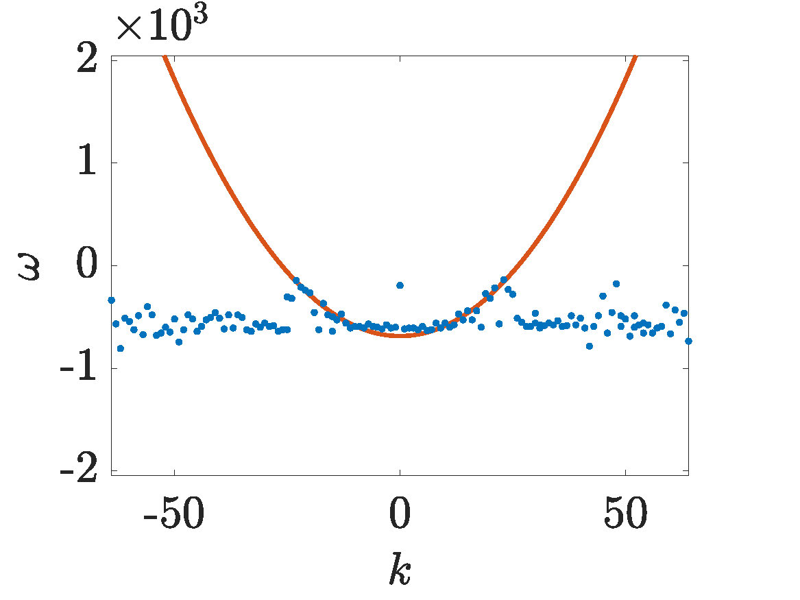
Figure 1. (animation Leisman-movie-1) This solution was propagated with focusing NLS from IC1, a perturbed standing wave with \(\gamma=0\) and amplitude \(A=12.7\). For this wave, modes \(|k|\le25\) will experience instability, because of this, most of the wave content is in those wave modes.

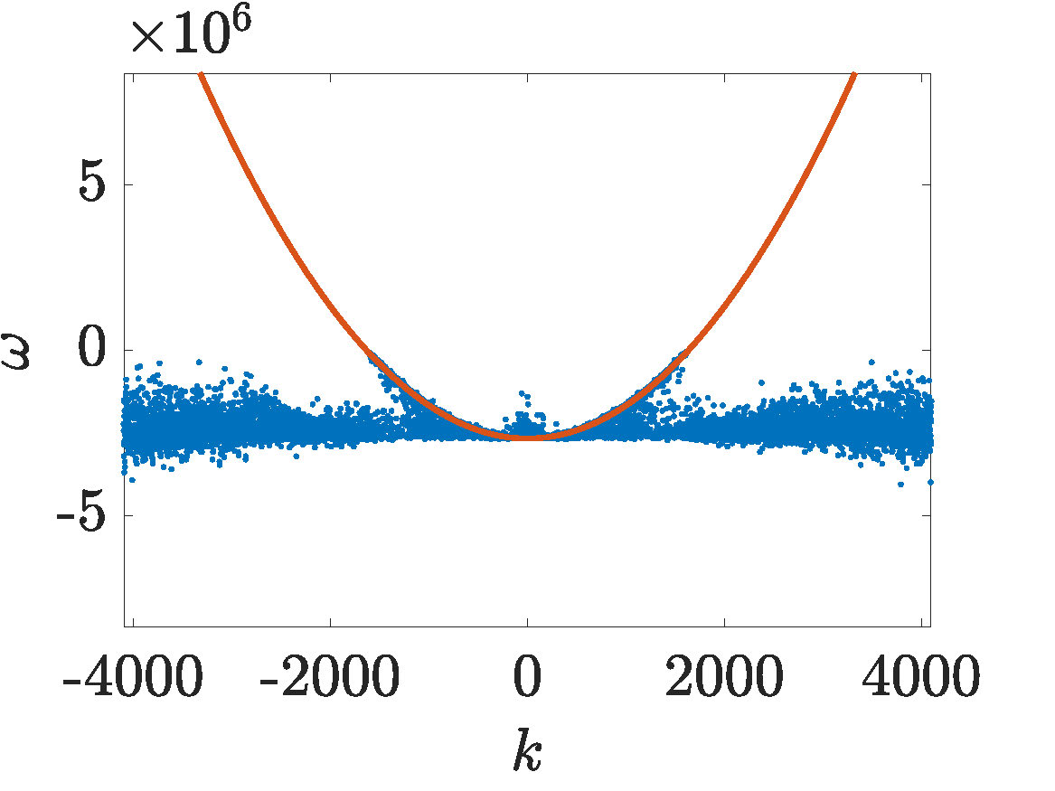
Figure 2. (animation Leisman-movie-2) This solution was propagated with focusing NLS from IC1, a perturbed standing wave with \(\gamma=0\) and amplitude \(A=814.6\). For this wave, modes \(|k|<1629\) will experience instability, because of this, most of the wave content is in those wave modes.

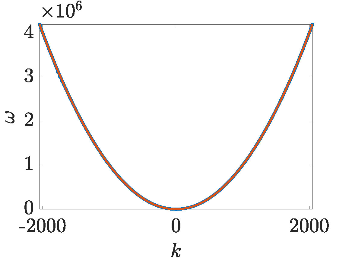
Figure 3. (animation Leisman-movie-3) This solution was propagated with focusing NLS from IC2, a smooth approximation to white noise with initial wave content in modes \(|k|<1629\), with mean amplitude \(A=24\). Most of the wave content remains in those modes \(|k|<1629\).

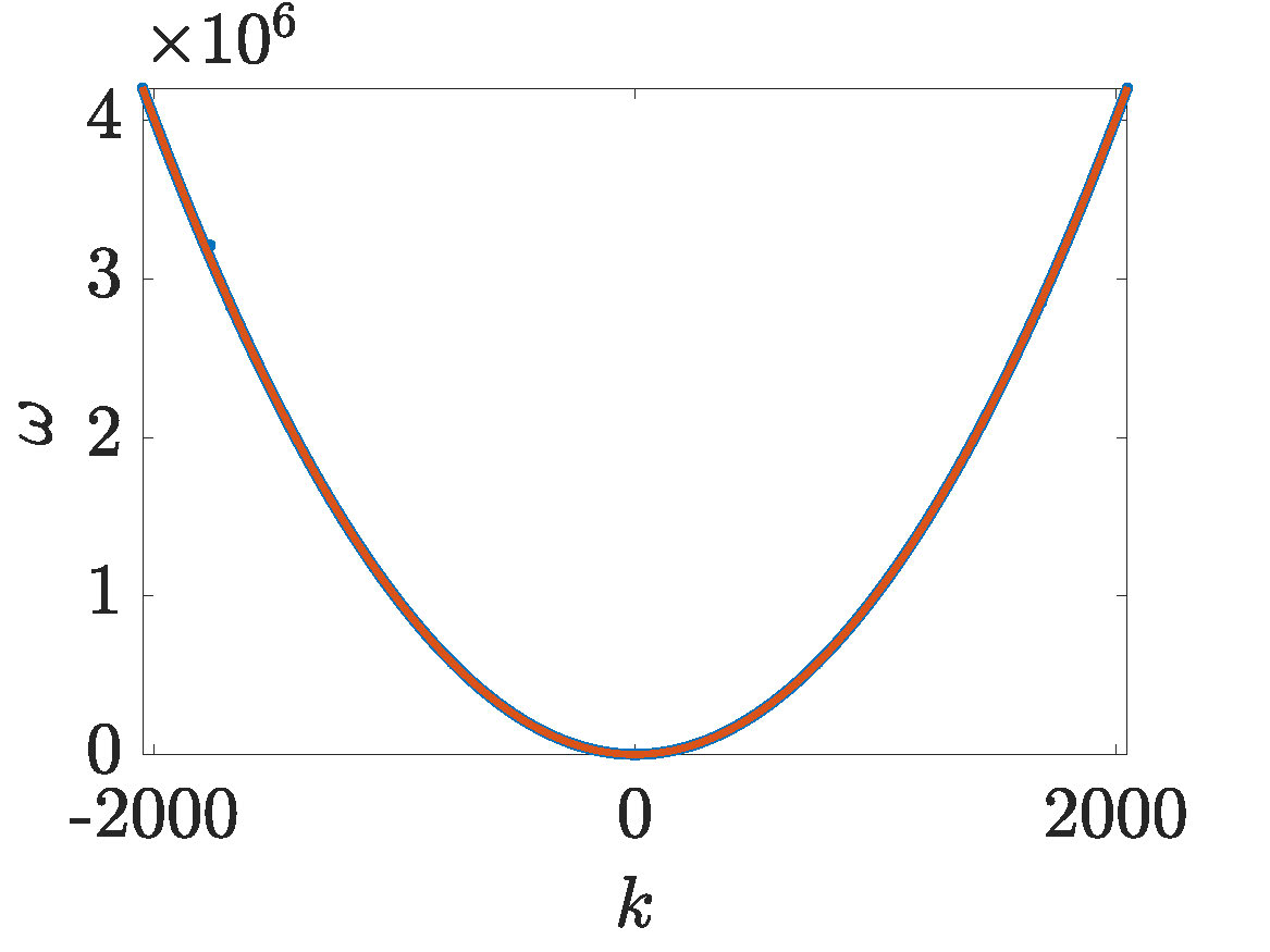
Figure 4. (animation Leisman-movie-4) This solution was propagated with defocusing NLS from IC2, a smooth approximation to white noise with initial wave content in modes \(|k|<1629\), with mean amplitude \(A=24\). Most of the wave content remains in those modes \(|k|<1629\).

4. Conclusion

In this article, we introduced the concept of an effective dispersion relation for nonlinear waves. We derived it analytically for the NLS under a weak nonlinearity assumption, and then showed a number of NLS waves with moderate to large amplitudes (thereby invalidating the assumption of weak nonlinearity), confirming that the same EDR still holds. In fact, while the examples shown here are only few, we have done this for a range of amplitudes of all three solution families, and even for some initial traveling waves. The following figure confirms excellent agreement between the measured parabola shift and the shift predicted from Eq. (9).

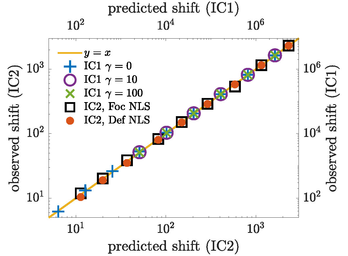
Figure 5. Scatter plot of the frequency shift \(\frac{4}{L}\|q(x,0)\|^2\) predicted by the EDR obtained in Eq. (9), versus the corresponding frequency shift observed using the WFS method, for increasing values of the wave norm \(\|q(x,0)\|\).

The main result here is that, for a robust family of waves, we found the parabolic EDR in Eq. (8), which equals the linear dispersion relation shifted by four times the total wave action of the wave.

Examples of observed or experimentally measured EDRs range over fields as diverse as surface gravity [19] and gravity-capillary waves [20], nonlinear springs [21], ionization waves [22], and graphene sheets [23]. Reference [20] presents a particularly striking example of an EDR with several distinct branches whose number depends on the amount of power injected into the waves. While none of these measurements have addressed EDRs for the NLS discussed here, experimental data yielding these EDRs may perhaps be obtained from observations and measurements of random and rogue waves in wave tanks [24, 25] and optics [26]. These are approximately described by the NLS, and our results may apply to them.

References

[1]   V. E. Zakharov and A. B. Shabat, Exact theory of two-dimensional self-focussing and one-dimensional self-modulating waves in nonlinear media, Soviet Journal of Experimental and Theoretical Physics, 34(1), 1972, pp. 62–69.

[2]   D. J. Benney and A. C. Newell, The propagation of nonlinear wave envelopes, Journal of Mathematics and Physics}, 46(1-4), 1967, pp. 133–139.

[3]   M. J. Ablowitz and H. Segur, Solitons and the Inverse Scattering Transform, SIAM, Philadelphia, 1981.

[4]   S. P. Novikov, S. V. Manakov, L. P. Pitaevskii, and V. E. Zakharov, Theory of Solitons: The Inverse Scattering Method, Plenum Press, New York, 1984.

[5]   L. D. Fadeev and L. A. Takhtajan, Hamiltonian Methods in the Theory of Solitons, Springer-Verlag, Berlin, 1987.

[6]   M. J. Ablowitz and P. A. Clarkson, Solitons, Nonlinear Evolution Equations and Inverse Scattering, Cambridge University Press, Cambridge, 1991.

[7]   C. Sulem and P.-L. Sulem, The Nonlinear Schrödinger Equation, Springer-Verlag New York, Inc., 1999.

[8]   M. J. Ablowitz, B. Prinari, and A. D. Trubatch, Discrete and continuous nonlinear Schrödinger systems, Cambridge University Press, volume 302, Cambridge, 2004.

[9]   G. B. Whitham, Linear and Nonlinear Waves, John Wiley & Sons, Inc, New York, 1974.

[10]   K. Plaisier Leisman, D. Zhou, J. W. Banks, G. Kovačič, and D. Cai, Effective dispersion in the focusing nonlinear schrödinger equation, Phys. Rev. E, 100, Aug 2019, p. 022215.

[11]   A. J. Majda, D. W. McLaughlin, and E. G. Tabak, A one-dimensional model for dispersive wave turbulence, Journal of Nonlinear Science, 7(1), 1997, pp. 9–44.

[12]   Y. Wakata, Frequency-wavenumber spectra of equatorial waves detected from satellite altimeter data, J. Oceanography, 63, 2007, pp. 483–490.

[13]   J. T. Farrar, Observations of the dispersion characteristics and meridional sea level structure of equatorial waves in the pacific ocean, J. Phys. Oceanography, 38(8), 2008, pp. 1669–1689.

[14]   T. Shinoda, G. N. Kiladis, and P. E. Roundy, Statistical representation of equatorial waves and tropical instability waves in the pacific ocean, Atmospheric Research, 94(1), 2009, pp. 37–44.

[15]   T. Shinoda, Observed dispersion relation of yanai waves and \(17\)-day tropical instability waves in the pacific ocean, SOLA, 6, 2010, pp. 17–20.

[16]   H. Hasimoto and H. Ono, Nonlinear modulation of gravity waves, Journal of the Physical Society of Japan, 33(3), 1972, pp. 805–811.

[17]   J. A. C. Weideman and B. M. Herbst, Split-step methods for the solution of the nonlinear schrödinger equation, SIAM Journal on Numerical Analysis, 23(3), 1986, pp. 485–507.

[18]   S. Filip, A. Javeed, and L. Trefethen, Smooth random functions, random odes, and gaussian processes, SIAM Review, 61(1), 2019, pp. 185–205.

[19]   T. H. C. Herbers, S. Elgar, N. A. Sarap, and R. T. Guza, Nonlinear dispersion of surface gravity waves in shallow water, Journal of Physical Oceanography, 32(4), 2002, pp. 1181–1193.

[20]   E. Herbert, N. Mordant, and E. Falcon, Observation of the nonlinear dispersion relation and spatial statistics of wave turbulence on the surface of a fluid, Phys. Rev. Lett., 105, Sep 2010, p. 144502.

[21]   K. L. Manktelow, M. J. Leamy, and M. Ruzzene, Analysis and experimental estimation of nonlinear dispersion in a periodic string, Journal of Vibration and Acoustics, 136(3), 2014, pp. 031016–031018.

[22]   K. Ohe, K. Asano, and S. Takeda, Nonlinear dispersion relation of finite amplitude ionisation waves. II. experiment, Journal of Physics D: Applied Physics, 14(6), 1981, pp. 1023–1029.

[23]   X. Jiang, H. Yuan, and X. Sun, Nonlinear plasmonic dispersion and coupling analysis in the symmetric graphene sheets waveguide, Scientific Reports, 6, 2016, p. 39309 EP.

[24]   M. Onorato, A. R. Osborne, M. Serio, and L. Cavaleri, Modulational instability and non-gaussian statistics in experimental random water-wave trains, Physics of Fluids, 17(7), 2005, p. 078101.

[25]   M. Onorato, A. R. Osborne, M. Serio, L. Cavaleri, C. Brandini, and C. T. Stansberg, Extreme waves, modulational instability and second order theory: wave flume experiments on irregular waves, European Journal of Mechanics - B/Fluids, 25(5), 2006, pp. 586–601.

[26]   M. Onorato, S. Residori, U. Bortolozzo, A. Montina, and F. T. Arecchi, Rogue waves and their generating mechanisms in different physical contexts, Physics Reports, 528(2), 2013, pp. 47–89.