G. Deng, Department of Mathematics and Statistics, 12 Wally's Walk, Macquarie University, New South Wales 2109, Australia.

1. Granular Chains

A granular chain is composed of tightly-packed frictionless aligned spherical particles. The following system of differential-difference equations govern the motion of a granular chain:

\( m(n)\ddot{x}(n,t)=\phi'(x(n+1,t)-x(n,t))-\phi'(x(n,t)-x(n-1,t)) \),

(1)

where \(n\in\mathbb{Z}\), \(m(n)\) is the mass of the \(n\)-th particle, \(x(n,t)\) is the position of the \(n\)-th particle at time \(t\), a dot denotes differentiation with respect to time, a prime denotes differentiation with respect to space, and the interaction potential between adjacent particles is

\( \begin{eqnarray} \phi(r)= \begin{cases} c(\delta-r)^{\alpha + 1}\,, &r\leq\delta \cr 0\,, &r>\delta \end{cases}\,, \quad c = \mathrm{constant} \end{eqnarray} \),

(2)

where \(\alpha > 1\) and \(\delta\) is the equilibrium overlap of adjacent particles due to the precompression that is induced by an external force. The interaction potential is zero when particles lose contact with each other. For algebraic convenience, we set \(c=1/(\alpha+1)\). In Figure 1, we illustrate a granular chain with precompression. The Hertzian interaction [9], which describes the behaviour of two contacting curved surfaces which deform slightly under stress, corresponds to \(\alpha = 3/2\). 

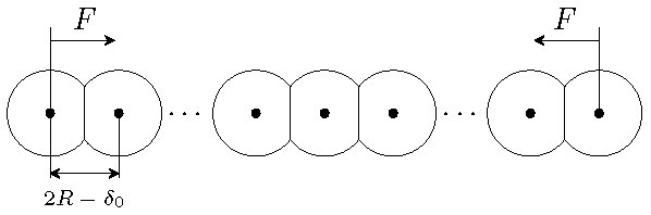
Figure 1. A particle chain with precompression. Force \(F\) at both ends compresses each sphere by a uniform distance \(\delta\).

Since the first prediction of solitary waves in granular chains [14], granular chains have been extensively studied [5, 15, 17], A significant feature of granular chains is their tunability. It is feasible to construct different types of perturbed granular chains experimentally by adding various heterogeneities to a homogeneous granular chain. For this review, we focus on woodpile chains [5, 6, 7, 11, 19], which is a type of perturbed granular chains and realizable in experiments. A woodpile chain consists of orthogonally stacked slender rigid cylinders [see Figure 2(a)]. The interaction force along the direction of the stack is determined by (2), and we can model the elastic deformation along the direction perpendicular to the stack direction using internal "resonators", where we determine the mass and coupling constant of these resonators based on the material and shape of the cylinders. When considering a stack of identical cylinders, each resonator has the same mass and elastic constant. We model such a woodpile chain as a monoatomic granular chain in which each particle with mass \(m_1\) is connected to an external particle with mass \(m_2\) by a linear spring with constant \(k\). We illustrate this woodpile chain model in Figure 2(b).

Woodpile chains behave in a fashion which is distinct from monatomic Hertizan chains. Typically, traveling-wave solutions in woodpile chains are not truly localized [6, 7, 11, 19]; instead, they take the form of a nanopteron [2].

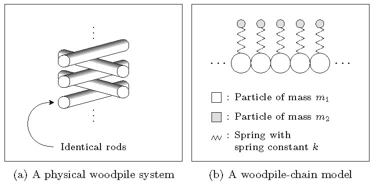
Figure 2. Panel (a) shows the physical configuration of orthogonal rods that is known as a "woodpile chain". Panel (b) shows an idealized model of the physical configuration in (a).

2. Nanoptera and Anti-Resonance Conditions

A nanopteron is the superposition of a central solitary wave and persistent oscillations on one or both sides of the central wave. The trailing oscillations typically have an exponentially small amplitude with respect to the singular perturbation parameter, which is the mass ratio in this example. Classical perturbation methods cannot capture the trailing oscillatory behavior. Recently, an exponential asymptotic method was applied to study exponentially small oscillations in diatomic chains [12, 13]. The exponential asymptotic analysis in [12, 13] was then extended to woodpile chains [6, 7]. They showed that the trailing oscillations in these perturbed systems are examples of the "Stokes' phenomenon", which refers to behavior that is switched on when Stokes curves are crossed in the complex plane.

Xu et al. [19] showed for uncompressed woodpile chains that trailing oscillations disappear for special parameter configurations, known as anti-resonance conditions. Performing exponential asymptotic analysis, [6] obtained anti-resonance conditions which are consistent with [19]. When anti-resonance conditions are satisfied, the solutions are true solitary waves. In [6, 12, 13], it was shown that anti-resonance conditions occur if nanoptera possess two Stokes curves which generate two distinct oscillations with the same amplitude but opposite phases.

3. Exponential Asymptotics

To find an asymptotic solution to a singularly perturbed differential equation, we determine some leading-order approximation \(g_0\) and expand the solution \(g\) about \(g_0\) as an asymptotic power series \(g \sim \sum_{j=0}^\infty \eta^{r j}g_j\) as \(\eta \rightarrow 0\), where \(r\) is the number of times that we need to differentiate \(g_{j-1}\) to obtain \(g_j\). If \(g_0\) has singular points, the series terms diverge in a factorial-over-power fashion [8]. Chapman et. al [4] proposed applying the following ansatz for late-order terms

\( g_j\sim\frac{G\Gamma(r j+\gamma)}{\chi^{r j+\gamma}}\quad \mathrm{as} \quad j\to\infty \),

(3)

where the parameter \(\gamma\) is constant and \(G\) and \(\chi\) are functions of any variables but are independent of \(j\).

In general, an asymptotic power series solution to a singularly perturbed problem is divergent [8]. If we truncate the series optimally so that the difference between the approximation and exact solution is minimum, the error is exponentially small [3]. We use \(N_{\mathrm{opt}}\) to denote an optimal truncation point. We then express the solution as

\( g = \sum_{j=0}^{N_{\mathrm{opt}}-1} \eta^{r j}g_j+g_{\exp} \).

(4)

Substituting (4) into the governing equation produces an equation for the exponentially small term \(g_{\exp}\) [16]. Away from Stokes curves, we determine \(g_{\exp}\) using the WKB method [10]. In the neighborhood of Stokes curves, we write

\( g_{\exp}\sim\mathcal{S}G\mathrm{e}^{-\chi/\eta} \quad \mathrm{as} \quad \eta \rightarrow 0 \),

(5)

where \(\mathcal{S}\) is known as the Stokes multiplier. The Stokes multiplier varies rapidly in the neighborhood of a Stokes curve and is constant elsewhere. This behavior is known as Stokes switching. The locations of Stokes curves are determined by \(\chi\). They occur where \(\chi\) is real and positive [1]. We can use exponential asymptotics to calculate the exponentially small contributions that appear as the Stokes curves are crossed.

4. Strongly Precompressed Woodpile Chains

We consider an idealized woodpile chain, as shown in Figure 2(b). We scale the system and obtain the governing equations

\( \ddot{u}(n,t) = [{\delta} + {u}(n-1,t) - {u}(n,t)]_+^\alpha - [{\delta} + {u}(n,t) - {u}(n+1,t)]_+^\alpha - {k} [{u}(n,t) - {v}(n,t)] \),

(6)

\( \eta^2 \ddot{{v}}(n,t) = {k} [{u}(n,t) - {v}(n,t)] \).

(7)

where \(u(n,t)\) and \(v(n,t)\) denote respectively the displacements of the \(n\)-th particle of mass \(m_1\) and \(m_2\) at time \(t\) and (\eta^2=m_2/m_1\). The subscript \(+\) indicates that we evaluate the bracketed term only if its argument is positive; it is equal to zero otherwise. To apply exponential asymptotic analysis we require \(0 < \eta \ll 1\).

The strongly precompressed woodpile chains are weakly nonlinear. Deforming (6)-(7) to the KdV equation, we obtain [14]

\( u_0(n,t)= -\frac{\delta\epsilon}{\alpha-1} \tanh\left(\epsilon(n-c_\epsilon t)\right) + \mathcal{O}(\epsilon^{3/2})\,,\quad u_0(n,t)=v_0(n,t)\,, \quad c_{\epsilon} = \delta^{(\alpha-1)/2} \sqrt{\alpha}+\frac{\sqrt{\alpha}}{6}\epsilon^2\delta^{(\alpha-1)/2} \).

(8)

where \(\epsilon\) quantifies the nonlinearity of the system. Defining \(\xi = n - c_{\epsilon} t\), we see that the leading-order behavior has singularities that are closest to the real axis at \(\xi_{\pm} = \pm\mathrm{i}\pi/2\epsilon\). The contributions from these singularities produce exponentially small oscillations.

Applying exponential asymptotic analysis, [7] shows that the traveling wave solution contains one Stokes curve across which trailing oscillations appear as shown in Figure 3. The amplitude of the trailing oscillations is obtained as

\( \mathrm{Amplitude} \sim\frac{2\delta \pi\sqrt{k}}{(\alpha-1)\eta c_{\epsilon}} \exp\left(-\frac{\pi\sqrt{k}}{2 c_{\epsilon}\epsilon\eta}\right) \quad \eta \rightarrow 0 \).

(9)

Note that the amplitude of the trailing oscillations is exponentially small in \(\eta\), but never zero. In Figure 4, we compare the asymptotic predictions and numerics.

5. Zero Precompression Woodpile Chains

The zero precompression system does not admit a linear limit and we cannot transform the system into the KdV equation. Instead we assume the leading-order behavior takes the form [18]

\( u_0(\xi) \approx \frac{A}{2}[1-\tanh(f(\xi)/2)],\quad f(\xi)=\sum_{j=0}^N C_{2j+1}\xi^{2j+1}, \quad \xi=j-c_A t \),

(10)

where \(A\) is the amplitude of the solitary wave, \(c_A\) is the velocity of the solitary wave with amplitude \(A\), and \(C_{2j+1}\) can be determined from numerics. Note that \(C_{2j+1}\) depends only on the interaction exponent \(\alpha\) in (2).

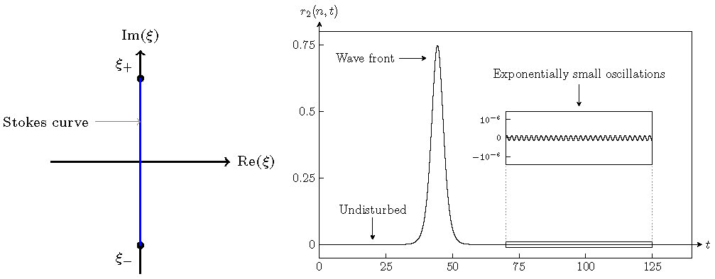
Figure 3. Left figure: the Stokes structure of the nanopteron solutions of (6)-(7). Right figure: numerically-calculated relative displacement of a light particle at some index \(n\) in a woodpile chain with \(\alpha=1.5\).

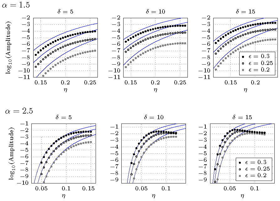
Figure 4. Comparison of asymptotic approximations and numerical simulations of the amplitude of exponentially small oscillations for woodpile chains with interaction exponents of (a) \(\alpha = 1.5\) and (b) \(\alpha = 2.5\).

The leading order has two singularity pairs that are closest to the real-axis. Hence the solution contains two Stokes curves as demonstrated in Figure 5, each of which generates one distinct set of oscillations. The amplitude of the total oscillation is given by [6]

\( \mathrm{Amplitude} \sim \frac{4|\bar{A}({\xi_{s}})| \pi\sqrt{k}}{\eta c_A} \exp\left(-\frac{\sqrt{k}\mathrm{Im}(\xi_s)}{c_A\eta}\right) \cos\left(\frac{\sqrt{k}\mathrm{Re}(\xi_s)}{c_A\eta}+\theta_{\xi_s}\right) \).

(11)

A comparison between asymptotic amplitude of the trailing oscillations and numerics is shown in Figure 6 for \(\alpha=1.5,2.5,3\). The anti-resonance conditions at which the trailing oscillations vanish correspond to the dips in Figure 6. These anti-resonance conditions agree with those predicted in [19].

6. Transition from the strongly nonlinear regime to weakly nonlinear regime

Woodpile chains with zero precompression permit anti-resonance conditions while woodpile chains with strong precompression do not. This difference can be understood by studying the behavior of the singularities in the leading order as we increase the precompression \(\delta\) [6] while fixing the leading-order amplitude. As we increase \(\delta\) the singularities move towards the imaginary axis and eventually coalesce, shown in Figure 7. For small values of \(\delta\), the solution contains two Stokes curves producing two oscillatory contributions. Once the value of \(\delta\) exceeds a particular value (in this case, approximately 0.284), the singularity pairs coalesce, and the solution has one Stokes curve, generating one oscillatory contribution, which can never be counteracted.

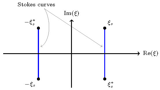
Figure 5. Stokes structure of traveling-wave solutions. Singularities that are closest to the real axis are represented by black dots and the corresponding Stokes curves are represented by solid blue curves.

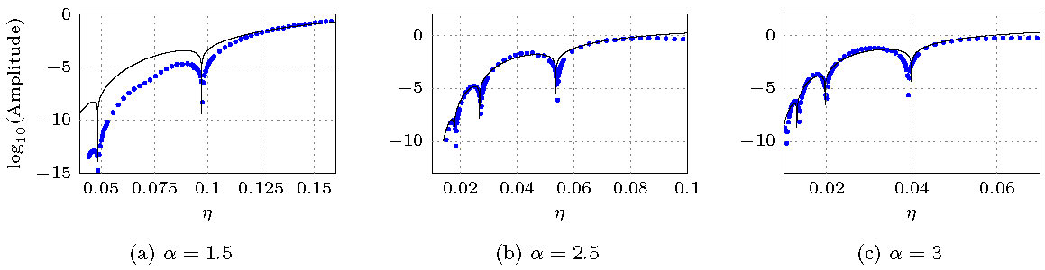
Figure 6. Comparison between asymptotic amplitude of trailing oscillations and numerics.

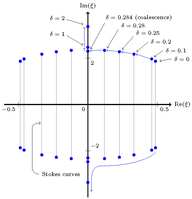
Figure 7. The singularity pairs in the complex plane for different values of the precompression \(\delta\), where the leading-order solitary wave has amplitude 5. Stokes lines extend vertically from the singularities, connecting the conjugate pairs.

References

[1]   M. V. Berry and C. J. Howls, Hyperasymptotics, Proc. Roy. Soc. Lond. A, 430(1880), 1990, pp. 653-668.

[2]   J. P. Boyd, A numerical calculation of a weakly non-local solitary wave: The \(\phi^4\) breather, Nonlinearity, 3(1), 1990, pp. 177-195.

[3]   J. P. Boyd, The devil's invention: Asymptotic, superasymptotic and hyperasymptotic series, Acta Appl. Math., 56(1), 1999, pp. 1-98.

[4]   S. J. Chapman, J. R. King, and K. L. Adams, Exponential asymptotics and Stokes lines in nonlinear ordinary differential equations, Proc. Roy. Soc. Lond. A, 454(1978), 1998, pp. 2733-2755.

[5]   C. Chong, M. A. Porter, P. G. Kevrekidis, and C. Daraio, Nonlinear coherent structures in granular crystals, J. Phys. Cond. Matt., 29(41), 2017, p. 413003.

[6]   G. Deng and C. J. Lustri, Nanoptera in nonlinear woodpile chains with zero precompression, arXiv:2105.02448, 2021.

[7]   G. Deng, C. J. Lustri, and M. A. Porter, Nanoptera in weakly nonlinear woodpile and diatomic granular chains, arXiv:2102.07322, 2021.

[8]   R. B. Dingle, Asymptotic Expansions: Their Derivation and Interpretation, Academic Press, New York, NY, USA, 1973.

[9]   H. Hertz, Üeber die berührung fester elastischer körper, J. Reine Angew. Math., 92(1881), pp. 156-171.

[10]   E. J. Hinch, Perturbation Methods, Cambridge Texts in Applied Mathematics, Cambridge University Press, Cambridge, UK, 1991.

[11]   E. Kim, F. Li, C. Chong, G. Theocharis, J. Yang, and P. G. Kevrekidis, Highly nonlinear wave propagation in elastic woodpile periodic structures, Phys. Rev. Lett., 114(11), 2015, p. 118002.

[12]   C. J. Lustri, Nanoptera and Stokes curves in the 2-periodic Fermi-Pasta-Ulam-Tsingou equation, Physica D, 402 (2020), p. 132239.

[13]   C. J. Lustri and M. A. Porter, Nanoptera in a period-2 Toda chain, SIAM J. Appl. Dyn. Syst., 17(2), 2018, pp. 1182-1212.

[14]   V. F. Nesterenko, Propagation of nonlinear compression pulses in granular media, J. Appl. Mech. Tech. Phy., 24 (1983), pp. 733-743.

[15]   V. F. Nesterenko, Dynamics of Heterogeneous Materials, Springer-Verlag, Heidelberg, Germany, 2001.

[16]   A. B. Olde Daalhuis, S. J. Chapman, J. R. King, J. R. Ockendon, and R. H. Tew, Stokes phenomenon and matched asymptotic expansions, SIAM J. Appl. Math., 55(6), 1995, pp. 1469-1483.

[17]   S. Sen, J. Hong, J. Bang, E. Ávalos, and R. Doney, Solitary waves in the granular chain, Phys. Rep., 462(2), 2008, pp. 21-66.

[18]   S. Sen and M. Manciu, Solitary wave dynamics in generalized hertz chains: An improved solution of the equation of motion, Phys. Rev. E, 64 (2001), p. 056605.

[19]   H. Xu, P. G. Kevrekidis, and A. Stefanov, Traveling waves and their tails in locally resonant granular systems, J. Phys. A Math. Theor., 48(19), 2015, p. 195204.