1. Sturm-Liouville theory and nodal domains

In one dimension, many dynamical stability problems can be reduced to the study of a Sturm-Liouville eigenvalue problem of the form

\( \frac{d}{dx} \left( p(x) \frac{du}{dx} \right) + q(x) u + \lambda r(x) u = 0, \)

on either the real line or a finite interval \((a,b)\) with appropriate boundary conditions. The application of such methods to the (in)stability of traveling waves is described in many places, for instance the textbook [KP13]. Here we restrict our attention to the interval \((a,b)\).

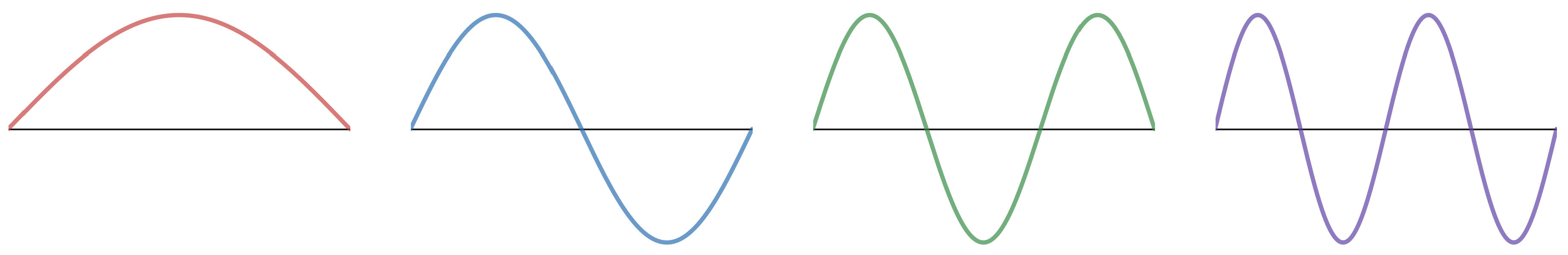
Figure 1. The first four eigenfunctions of a Sturm-Liouville problem (with Dirichet boundary conditions). The \(n\)th eigenfunction has \(n-1\) interior zeros, and provides a partition into \(n\) nodal domains.

A well known theorem, due to Sturm, says there is a countable sequence of eigenfunctions, \(u_1, u_2, \ldots\), with the property that \(u_n\) has exactly \(n-1\) zeros in the open interval \((a,b)\). These \(n-1\) zeros partition the interval \((a,b)\) into \(n\) nodal domains-- connected sets on which \(u_n\) is strictly positive or strictly negative. See Figure 1 for an illustration of this qualitative behaviour.

The reformulation of Sturm's result in terms of nodal domains is convenient when one considers more than one spatial dimension, in which case there are infinitely many zeros, but the number of nodal domains remains finite. This is the basis for Courant's nodal domain theorem, which says that the \(n\)th eigenfunction of the Laplacian (or any other second-order, self-adjoint, elliptic operator) has at most \(n\) nodal domains.

Returning to one dimension, it is also possible to partition \((a,b)\) using the critical points, rather than zeros, of an eigenfunction. This gives a partition into subintervals on which the eigenfunction satisfies Neumann boundary conditions, meaning its derivative vanishes at the endpoints of each subinterval.

The generalization of this latter partition to higher dimensions is less obvious -- while one can immediately define the zero set of a function (which forms the boundary of its nodal domains), it is not as straightforward to find a hypersurface along which the normal derivative vanishes, since the normal direction depends on the hypersurface itself. This can be resolved using constructions from dynamical systems, namely the theory of invariant manifolds, which we describe next.

2. Invariant manifolds and Neumann domains

For simplicity we only describe the construction on the 2-torus, \(\mathbb{T}^2\), by working on \(\mathbb{R}^2\) and assuming that all functions under consideration are \(2\pi\)-periodic in both \(x\) and \(y\). Thus let \(f \colon \mathbb{R}^2 \to \mathbb{R}\) be smooth and periodic. We assume that \(f\) is a Morse function. This means at each critical point \(p\), where \(\nabla f(p) = 0\), the Hessian matrix of second partials

\( \text{Hess} f(p) = \begin{bmatrix} f_{xx}(p) & f_{xy}(p) \\ f_{yx}(p) & f_{yy}(p) \end{bmatrix} \)

is invertible. This is a reasonable assumption to impose, as we are primarily interested in eigenfunctions, and it is known that these are generically Morse [Uhl76].

For such an \(f\) we let \(\varphi(t,x)\) denote the (negative) gradient flow. That is, for each \(x \in \mathbb{R}^2\), \(\varphi(t,x)\) solves the initial value problem

\( \frac{d}{dt} \varphi(t,x) = - \nabla f (\varphi(t,x)), \quad \varphi(0,x) = x. \)

For each critical point \(p\) we define the stable and unstable manifolds by

\( W^{s}(p) = \Big\{x : \lim_{t\rightarrow\infty} \varphi(t,x) = p\Big\} \)

and

\( W^{u}(p) = \Big\{x : \lim_{t\rightarrow-\infty} \varphi(t,x) = p \Big\}, \)

respectively.

Definition 1. Suppose \(f\) has a minimum at \(p\) and a maximum at \(q\), and \(W^s(p) \cap W^u(q)\) is nonempty. Each connected component of \(W^s(p) \cap W^u(q)\) is called a Neumann domain.

These can be thought of topographically. If \(f\) is a "height function" describing the altitude of some mountainous terrain, maxima correspond to summits, and minima correspond to points of lowest elevation (which are called "immits" by Cayley [Cay59] and "bottoms" by Maxwell [Max70]). Continuing this analogy, Maxwell calls the stable manifold of a minimum a "basin" or "dale," and the unstable manifold of a maximum a "hill."

Another important concept is a Neumann line, which is the closure of a flow line which has (at least) one endpoint at a saddle. The union of all Neumann lines is called the Neumann line set, and it is not hard to show that \(\mathbb{T}^2\) is the disjoint union of its Neumann domains and the Neumann line set.

Maxwell [Max70] calls such a line a watershed if it ends at a summit, and a watercourse if it ends at a bottom. He then says:

Lines of Watershed are the only lines of slope which do not reach a bottom, and lines of Watercourse are the only lines of slope which do not reach a summit. All other lines of slope diverge from some summit and converge to some bottom, remaining throughout their course in some district belonging to that summit and that bottom, which is bounded by two watersheds and two watercourses.

A moment's reflection reveals that the "district belonging to that summit and that bottom" is precisely a Neumann domain as defined above.

As a first example, consider the function \(f(x,y) = \sin x \sin y\), for which we take \([0,2\pi) \times [0,2\pi)\) as a fundamental domain. This has eight critical points:

• maxima at \((\frac{\pi}{2}, \frac{\pi}{2})\) and \((\frac{3\pi}{2}, \frac{3\pi}{2})\);
• minima at \((\frac{\pi}{2}, \frac{3\pi}{2})\) and \((\frac{3\pi}{2}, \frac{\pi}{2})\);
• saddle points at \((0,0)\), \((0,\pi)\), \((\pi,0)\) and \((\pi,\pi)\).

The critical points, and the corresponding Neumann lines, which partition the torus into eight Neumann domains, are shown in Figure 2. (When counting critical points and Neumann domains, recall that the top and bottom of the square are identified, as are the left and right sides.)

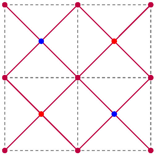
Figure 2. The nodal domains and Neumann domains for the function \(f(x,y) = \sin x \sin y\), illustrated on \([0,2\pi] \times [0,2\pi]\). Minima and maxima are denoted by blue and red dots, respectively, and saddle points are denoted by purple dots. The nodal set (i.e., zero set) is denoted by a dashed gray line, and the Neumann set is indicated by a solid purple line.

In this first example, the Neumann lines always intersect at right angles. While this will always be true at a saddle, at an extrema they will in general intersect at angles 0 and \(\pi\), as seen in our second example, Figure 3. This means the boundary of a Neumann domain can have cusps, which complicates their study. Fortunately this difficulty can be overcome using tools from dynamical systems, in particular the Hartman-Grobman theorem.

The decomposition of a manifold into Neumann domains has appeared in many different contexts over the years, going back at least as far as the 1870 paper of Maxwell described above. They have recently made an appearance as a valuable tool in image segmentation, shape analysis and data analysis; see, for instance, [RM00,EHVP03,EHZ03,GBP12] and the survey [EH08]. In these references the collection of Neumann domains is usually referred to as a Morse-Smale complex, and is considered under the slightly more restrictive assumption that \(f\) is a Morse-Smale function. Morse-Smale complexes also play a significant role in Morse homology and Floer homology [BH04], the latter arising from Arnold's conjecture on the number of periodic orbits of a Hamiltonian system [Sal99].

In the context of Sturm-Liouville theory and the decomposition into nodal domains of an eigenfunction, this kind of construction was first hinted at in [CFZ97], and later developed in [McD08] and [MF14]. It was also suggested independently in the survey article [Zel13].

We use the name Neumann domain for the following reason. Since the boundary of each Neumann domain consists of gradient flow lines, it is always tangent to \(\nabla f\), and so the normal derivative vanishes,

\( \frac{\partial f}{\partial n}\bigg|_{\partial\Omega} = 0, \)

at any point where the boundary is smooth enough to have a well-defined normal.

Therefore, given a function \(f\), we have exhibited a decomposition of its domain into sets on which \(f\) satisfies Neumann boundary conditions, analogous to the decomposition into nodal domains. The rest of this article will describe relevant properties of Neumann domains and Neumann lines, as well as some accompanying spectral theory, emphasizing the roles of dynamical systems techniques.

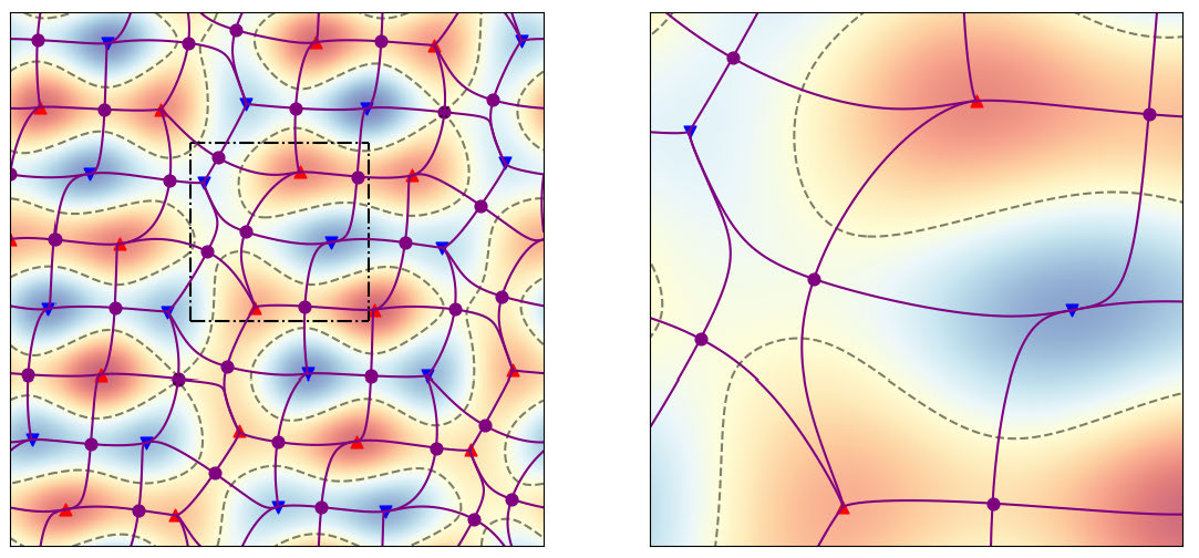
Figure 3. An eigenfunction corresponding to the eigenvalue \(\lambda=17\) on the torus (left), and a magnification (right). Circles mark saddle points and triangles mark extrema (maxima by triangles pointing upwards and vice versa for minima). The nodal set is represented by a dashed line and the Neumann line set is marked by solid purple lines. (Figure produced by Sebastian Egger using [Tay18]).

3. Geometric and topological properties

Fundamental geometric and topological properties of Neumann domains were established in [MF14] and [BF16]; see also [ABBE20] for a recent survey. We review some of the most important ones here, emphasizing the structure of the Neumann lines that form the boundary.

Every critical point of \(f\) is contained in the Neumann line set. Moreover, recalling that a Neumann domain \(\Omega\) is a connected component of \(W^s(p) \cap W^u(q)\), the only extrema on the boundary are \(p\) and \(q\) themselves. Therefore, \(\partial\Omega\) consists of flow lines connecting \(p\), \(q\), and some number of saddle points.

If all of the stable and unstable manifolds intersect transversely, \(f\) is said to be Morse-Smale. In two dimensions it is not hard to see that this is equivalent to the absence of flow lines between two saddle points. In this case every flow line connects a saddle to either \(p\) and \(q\), which means there must be either one or two saddles on the boundary of \(\Omega\).

A Neumann domain with just one saddle on the boundary, as shown in Figure 4(right), is rather degenerate, as the boundary has a "crack" (the curve \(\eta\)) with the property that \(\Omega\) lies on both sides, and this makes it poorly behaved from the perspective of boundary value problems. It is not known if there exist eigenfunctions with such Neumann domains, but it is possible to construct Morse-Smale functions with this property; see [BCE20, Appendix A] for details.

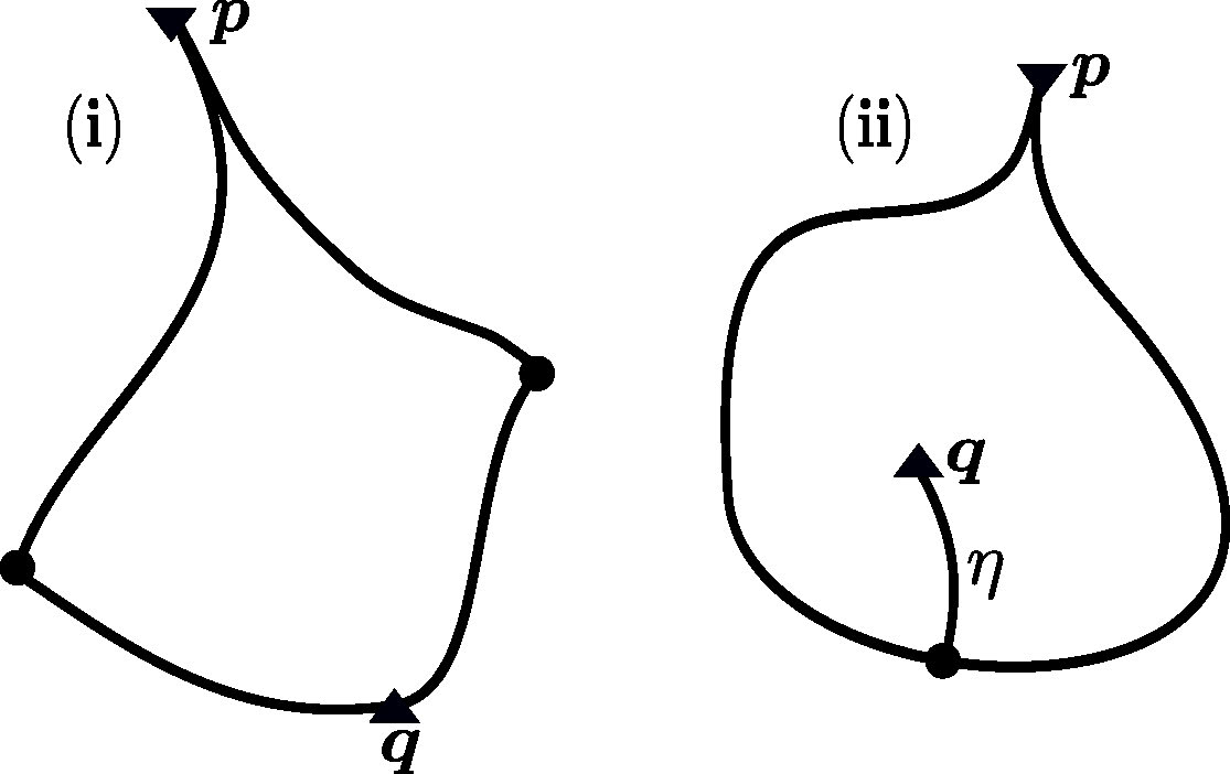
Figure 4. Neumann domains with either two or one saddles on the boundary. Saddle points are represented by balls, maxima by triangles pointing upwards and vice versa for minima.

At a saddle point four Neumann lines meet, with the angle between any two adjacent lines being \(\pi/2\). On the other hand, at an extrema for which the Hessian has distinct eigenvalues, Neumann lines must meet with angle 0, \(\pi/2\) or \(\pi\), with \(\pi/2\) being exceptional (see Figure 3).

It follows that the boundary of a Neumann domain could have a cusp (when the meeting angle is 0) and so it can fail to be Lipschitz continuous. Furthermore, the Neumann domain can even fail to be continuous. This may seem counterintuitive, as the boundary appears to be (and indeed is!) a continuous curve. However, by definition a domain is continuous if its boundary can locally be represented (after a suitable rotation) by the graph of a continuous function, and this need not hold at a cusp; see Figure 5 for an example and [EE87,MP01] for further discussion.

The presence of cusps and cracks makes the analysis of Neumann domains significantly more complicated than their nodal counterparts. (While a nodal domain may have irregular boundary, the Dirichlet boundary conditions make this irrelevant. In analytic terms: the Sobolev space \(H^1(\Omega)\) is much more sensitive to the geometry of \(\partial\Omega\) than \(H^1_0(\Omega)\) is.)

4. Further geometric structure via Hartman's theorem

To study differential equations (and in particular eigenvalue problems) on a Neumann domain, we need more a more refined description of its boundary in the vicinity of a cusp. We first recall the Hartman-Grobman theorem, as it appears in most textbooks.

Theorem 2. Suppose \(F \colon \mathbb{R}^d \to \mathbb{R}^d\) is smooth and let \(\varphi(t,x)\) denote the flow of the (nonlinear) system \(\dot x = F(x)\). Suppose \(p\) is a hyperbolic equilibrium, i.e., \(F(p) = 0\) and \(DF(p)\) has no eigenvalues on the imaginary axis. Then there exists a homeomorphism \(\Phi:U\rightarrow V\) from an open neighbourhood \(U\) of \(p\) onto an open neighbourhood \(V\) of the origin, such that for each \(x\in U\) the flow line through \(x\) is given by

\( \varphi(t,x) = \Phi^{-1} \big(e^{DF(p)t}\Phi(x)\big) \)

for sufficiently small \(t\).

In other words, near \(p\) the flow of the original nonlinear system is (topologically) equivalent to the flow of the linearized system, which can be calculated explicitly.

For the gradient flow of a Morse function, with \(F = -\nabla f\), the hypotheses of the theorem are automatically satisfied, because \(DF(p) = - \text{Hess} f(p)\) is symmetric and non-degenerate, hence its eigenvalues are non-zero real numbers. For instance, suppose \(p\) is a minimum, and \(\text{Hess} f(p)\) has eigenvalues \(0 < \lambda_1 \leq \lambda_2\). Assuming for simplicity that \(\text{Hess} f(p) = \operatorname{diag}( \lambda_1, \lambda_2)\), as can always be arranged by a suitable rotation of coordinates, a trajectory of the linearized system will then be of the form

\( \begin{bmatrix} x(t) \\ y(t) \end{bmatrix} = e^{-t \text{Hess} f(p)} \begin{bmatrix} x_0 \\ y_0 \end{bmatrix} = \begin{bmatrix} e^{-\lambda_1 t} x_0 \\ e^{-\lambda_2 t} y_0 \end{bmatrix} \)

for some \((x_0,y_0) \in \mathbb{R}^2\), which implies

\( y(t) = c_0 x(t)^\alpha, \)

where \(\alpha = \lambda_2/\lambda_1 \geq 1\) and \(c_0 = y_0 / x_0^\alpha\). Note that \(\alpha\) depends only on the Hessian eigenvalues, and is independent of the starting point \((x_0,y_0)\).

Now suppose \(p\) is on the boundary of some Neumann domain \(\Omega\). Near \(p\), it follows that the flow lines forming the boundary of \(\Omega\) can be described (in this new coordinate system) by \(y = c_1 x^\alpha\) and \(y = c_2 x^\alpha\), for some constants \(c_1\) and \(c_2\). The Hartman-Grobman theorem therefore allows us to transform \(\Omega\) into the "normal form" or "model domain"

\( \tilde\Omega = \big\{ (x,y) : 0 < x < 1 \text{ and } c_1 x^\alpha < y < c_2 x^\alpha \big\} \)

in a neighbourhood of \(p\). See Figure 5 for two examples of such a domain, one where \(c_1\) and \(c_2\) have the same sign, and one where they have opposing signs.

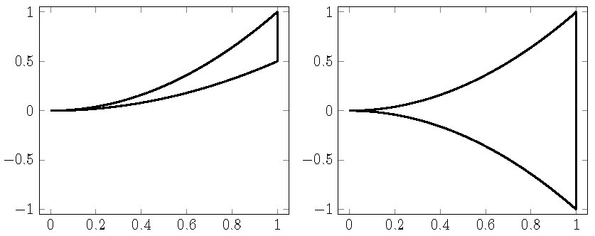
Figure 5. The regions \(\{\frac12 x^2 < y < x^2 \}\) (left) and \(\{ - x^2 < y < x^2 \}\) (right).

Unfortunately, this version of the theorem is not adequate for studying Neumann domains. The problem is that to analyze solutions of a differential equation on a Neumann domain \(\Omega\), one needs to know how their derivatives transform when mapped onto the model domain \(\tilde\Omega\). This means the map \(\Phi\), and its inverse, should be continuously differentiable.

It is well known that a continuous homeomorphism \(\Phi\) is the most one can expect in general; see, for instance, [Per01] or [Chi06] for examples and further discussion. However, there are several situations in which \(\Phi\) is guaranteed to be a \(C^1\) diffeomorphism:

• when the dimension \(d=2\);
• when the eigenvalues of \(DF(p)\) are all in the same half-plane;
• when the eigenvalues of \(DF(p)\) satisfy a certain Diophantine inequality.

In the present setting either of the first two results (both of which are due to Hartman [Har60]) will suffice, since we are only considering planar systems, and cusps can only occur at minima or maxima, where the Hessian is sign definite. See [CS00] for a modern exposition of these results.

Before moving on, we mention that the question of further differentiability of \(\Phi\) (which becomes relevant when studying regularity of weak solutions of differential equations on a Neumann domain) is much more subtle. For instance, Sternberg has given an example of an analytic planar system which cannot be linearized by a \(C^2\) diffeomorphism [Ste57].

5. Spectral theory of Neuman domains

We finish by describing some of the spectral theory of Neumann domains, again motivated by the analogy with nodal domains and Sturm-Liouville theory.

If \(f\) is an eigenfunction, and \(U\) is one of its nodal domains, then the restriction \(f\big|_U\) will vanish on the boundary \(\partial U\) and satisfy the same eigenvalue equation. Therefore, it is an eigenfunction for the Dirichlet problem on \(U\). Moreover, since it never vanishes in \(U\), it must be the first eigenfunction. This fact plays a crucial role in the study of nodal domains, and many fundamental results, such as Courant's nodal domain theorem, rely on it.

It is therefore natural to consider the restriction of \(f\) to one of its Neumann domains, \(\Omega\). As described above, the normal derivative vanishes on the smooth parts of the boundary, so \(f\big|_\Omega\) is expected to be an eigenfunction for the Neumann problem on \(\Omega\). While this is indeed the case, it is nontrivial to verify. Due to the potential irregularity of the boundary, in particular the presence of cracks and cusps, the Neumann boundary conditions must be interpreted in a distributional sense, and so it is not obvious that they are actually satisfied. This was recently verified in [BCE20], using Hartman's theorem as described in the previous section.

Now that we know \(f\big|_\Omega\) is an eigenfunction of the Neumann problem on \(\Omega\), we would like to ask which eigenfunction it is. However, there is an additional complication to be overcome first: While the spectrum of the Dirichlet problem on an arbitrary open set consists entirely of isolated eigenvalues of finite multiplicity, the same need not be true for the Neumann problem. Indeed, the essential spectrum may be nonempty, and in fact can be an arbitrary closed subset of \([0,\infty)\), as was shown in [HSS91].

Nevertheless, on a Neumann domain one can use Hartman's theorem to show that the spectrum of the Neumann problem is discrete, i.e., is just a countable sequence of isolated eigenvalues, so we can indeed ask which of these the restricted eigenfunction \(f\big|_\Omega\) corresponds to.

However, unlike the case of nodal domains, this restriction will never be the first Neumann eigenfunction on \(\Omega\). This can be seen from Figure 3, which shows that the restricted function changes sign on each Neumann domain, whereas the first eigenfunction must be sign definite (in fact it is just a constant). A reasonable guess is that it is instead the second eigenfunction, but this is not true either, and in fact the restricted eigenfunction can appear anywhere in the spectrum of the Neumann problem on \(\Omega\). More precisely, it was shown in [BET20] that for any natural number \(n\) there exists an eigenfunction \(f\) on \(\mathbb{T}^2\), and a Neumann domain \(\Omega\) of \(f\), such that \(f\big|_\Omega\) is the \(n\)th (or possibly higher) eigenfunction for the Neumann problem on \(\Omega\). In other words, \(f\big|_\Omega\) is not among the first \(n-1\) eigenfunctions on \(\Omega\).

There are few general results about the spectral position of an eigenfunction, or the number of Neumann domains it may have. We refer the reader to [ABBE20] for a short but comprehensive review of what is currently known.

6. Summary

In this article we partitioned the torus into Neumann domains of a given function, analogous to the nodal domain decomposition but with Neumann conditions on the boundary instead of Dirichlet. The boundary of a Neumann domain can be irregular, having both cracks and cusps, but the resulting analytic difficulties can be overcome using tools from dynamical systems, in particular the \(C^1\) version of the Hartman-Grobman theorem. The spectral theory of Neumann domains is much more involved than the corresponding Dirichlet case, and many interesting open problems remain.

Acknowledgments

This work was supported by NSERC grant RGPIN-2017-04259.

References

[ABBE20]   L. Alon, R. Band, M. Bersudsky, and S. Egger, Neumann domains on graphs and manifolds, Analysis and Geometry on Graphs and Manifolds, London Math. Soc. Lecture Note Ser., vol. 461, Cambridge Univ. Press, 2020, pp. 203-249.

[BCE20]   R. Band, G. Cox, and S. K. Egger, Defining the spectral position of a Neumann domain, https://arxiv.org/abs/2009.14564, 2020.

[BET20]   R. Band, S. Egger, and A. Taylor, The spectral position of Neumann domains on the torus, J. Geom. Anal., https://doi.org/10.1007/s12220-020-00444-9, 2020.

[BF16]   R. Band and D. Fajman, Topological properties of Neumann domains, Ann. Henri Poincaré, 17 (2016), pp. 2379-2407.

[BH04]   A. Banyaga and D. Hurtubise, Lectures on Morse homology, Kluwer Academic Publishers Group, 2004.

[Cay59]   A. Cayley, On contour and slope lines, The London, Edinburgh, and Dublin Philosophical Magazine and Journal of Science, 18 (1859), no. 120, pp. 264-268.

[CFZ97]   G. Chen, S. A. Fulling, and J. Zhou, Asymptotic equipartition of energy by nodal points of an eigenfunction, J. Math. Phys., 38 (1997), no. 10, pp. 5350-5360. MR 1471933.

[Chi06]   C. Chicone, Ordinary differential equations with applications, second ed., Texts in Applied Mathematics, vol. 34, Springer, New York, 2006. MR 2224508.

[CS00]   C. Chicone and R. Swanson, Linearization via the Lie derivative, Electronic Journal of Differential Equations. Monograph, vol. 02, Southwest Texas State University, San Marcos, TX, 2000. MR 1804049.

[EE87]   D. E. Edmunds and W. D. Evans, Spectral theory and differential operators, Oxford University Press, 1987.

[EH08]   H. Edelsbrunner and J. Harer, Persistent homology--a survey, Surveys on discrete and computational geometry, Contemp. Math., vol. 453, Amer. Math. Soc., Providence, RI, 2008, pp. 257-282. MR 2405684.

[EHNP03]   H. Edelsbrunner, J. Harer, V. Natarajan, and V. Pascucci, Morse-Smale complexes for piecewise linear 3-manifolds, Proceedings of the Nineteenth Annual Symposium on Computational Geometry (New York, NY, USA), SCG '03, Association for Computing Machinery, 2003, pp. 361–370.

[EHZ03]   H. Edelsbrunner, J. Harer, and A. Zomorodian, Hierarchical Morse-Smale complexes for piecewise linear 2-manifolds, Discrete Comput. Geom., 30 (2003), no. 1, pp. 87-107, ACM Symposium on Computational Geometry (Medford, MA, 2001). MR 1991588.

[GBP12]   A. Gyulassy, P. Bremer, and V. Pascucci, Computing Morse-Smale complexes with accurate geometry, IEEE Transactions on Visualization and Computer Graphics, 18 (2012), no. 12, pp. 2014-2022.

[Har60]   P. Hartman, On local homeomorphisms of Euclidean spaces, Bol. Soc. Mat. Mexicana (2), 5 (1960), pp. 220-241. MR 141856.

[HSS91]   R. Hempel, L. Seco, and B. Simon, The essential spectrum of Neumann Laplacians on some bounded singular domains, J. Funct. Anal., 102 (1991), pp. 448-483.

[KP13]   T. Kapitula and K. Promislow, Spectral and dynamical stability of nonlinear waves, Applied Mathematical Sciences, vol. 185, Springer, New York, 2013, With a foreword by Christopher K. R. T. Jones. MR 3100266.

[Max70]   J. C. Maxwell, On hills and dales, The London, Edinburgh, and Dublin Philosophical Magazine and Journal of Science, 40 (1870), no. 269, pp. 421-427.

[McD08]   R. B. McDonald, Neumann bounded partitions of eigenfunctions, Undergraduate thesis, Texas A&M University, 2008.

[MF14]   R. McDonald and S. Fulling, Neumann nodal domains, Philos. Trans. R. Soc. Lond. Ser. A Math. Phys. Eng. Sci., 372 (2014), 20120505, 6.

[MP01]   V. G. Maz'ya and S. V. Poborchi, Differentiable functions on bad domains, World Scientific Publishing, 2001.

[Per01]   L. Perko, Differential equations and dynamical systems, Springer-Verlag, 2001.

[RM00]   J. B. T. M. Roerdink and A. Meijster, The watershed transform: definitions, algorithms and parallelization strategies, Fund. Inform., 41 (2000), no. 1-2, pp. 187-228. MR 1773369.

[Sal99]   D. Salamon, Lectures on Floer homology, Symplectic geometry and topology (Park City, UT, 1997), IAS/Park City Math. Ser., vol. 7, Amer. Math. Soc., Providence, RI, 1999, pp. 143-229. MR 1702944.

[Ste57]   S. Sternberg, Local contractions and a theorem of Poincaré, Amer. J. Math., 79 (1957), pp. 809-824. MR 96853.

[Tay18]   A. J. Taylor, pyneumann toolkit, https://github.com/inclement/neumann, 2018.

[Uhl76]   K. Uhlenbeck, Generic properties of eigenfunctions, Amer. J. Math., 98 (1976), pp. 1059-1078.

[Zel13]   S. Zelditch, Eigenfunctions and nodal sets, Surveys in differential geometry. Geometry and topology, Surv. Differ. Geom., vol. 18, Int. Press, Somerville, MA, 2013, pp. 237-308. MR 3087922.