Olivia Cannon: joint work with Ty Bondurant, Malindi Whyte, and Arnd Scheel.
Social Dynamics and `Bounded Confidence'
If social media, middle schoolers, or the last few years have taught us anything, it is that group opinion dynamics can be wild - and are perhaps poorly understood. But understanding even how individual opinions change through the lens of mathematics is a relatively new (at least as a prominent field, on the order of the lifetime of the author of this DSWeb article), multifaceted, and exciting field of study (interested readers should see the work of many, including but not limited to, Mason Porter, Heather Zinn-Brooks, Juan G. Restrepo, Al Volkening, Javier Gomez-Serrano, and many more).
How does one study such a thing? Even understanding how a population's opinion on one given topic evolve would be deeply valuable, so one could consider such a population, expressing each agent's opinion as a number. (We do this often in real life ourselves with rating systems, even). One then lets agents interact, and devises rules for how interaction of people with differing opinions affects them.
A famous and important tenet is that all models are wrong - but the best ones, perhaps, capture something important. In the early 2000, Deffuant and Weisbach [6], as well as Hegselmann and Krause [11] proposed models which shared the following principle:
People interact, and compromise their opinions - but they only compromise
with those whose opinions are sufficiently close in the first place.
This idea became the foundation for a family of models called bounded confidence models, which have become seminal in the field of opinion dynamics.
The present work [2] begins with a bounded confidence model on a lattice. Opinions are taken to be integer-valued, and the population \(P_n\) with opinion \(n\) evolves according to
| |
\( \frac{dP_n}{dt} = 2P_{n+1}P_{n-1} - P_n(P_{n+2} + P_{n-2}), \qquad P_n\geq 0, \ n\in\mathbb{Z}. \) |
(0.1) |
Agents with opinions \(n-1\) and \(n+1\) each compromise to opinion \(n\), and agents with opinion \(n\) compromise with those with opinion \(n-2\) and \(n+2\). Note that (0.1) is deterministic, modeling the opinion distribution of a population over time. It is also spatially extended; opinions may take any integer value.
The dynamics of various bounded confidence models can differ, but a key feature common to many is the evolution of opinions toward one or more clustered states. In (0.1), the uniform state, where the population is equally distributed between each opinion, is unstable, and small perturbations lead to the formation of regularly-spaced clusters.
A simulation of (0.1) from a small perturbation of a uniform state.
Adding Bias
Bounded confidence models are a natural tool to study mechanisms of polarization, and to that end, many modifications have been studied, including for instance variations of the confidence interval between agents, introduction of a small number of agents who do not compromise (`stubborn' agents), and variations in the probability of interaction [4, 5, 7, 8, 10, 12, 13, 14, 15]. Along a slightly different vein, however, the present work concerns the drift of opinion clusters; that is, the continuous movement of clusters toward one extreme of the opinion spectrum.
The driving motivation of our project was the following:
Do there exist bias terms which cause existing opinion clusters to shift continuously, while also staying together?
This question is both mathematical and phenomenological. Anyone with a traveling-waves background may recognize it as asking, in some sense, can we find `traveling waves' of opinions? But one also wants to think from a modeling perspective - what would such a bias term come from sociologically?
Self-Incitement: A Tale of Three Models
We consider equations of the form
| |
\( \frac{dP_n}{dt} = 2P_{n+1}P_{n-1} - P_n(P_{n+2} + P_{n-2}) + \beta G(P)_n, \qquad P_n\geq 0, \ n\in\mathbb{Z}, \) |
(0.2) |
where \(\beta G(P)\) represents the bias term. The parameter \(\beta\) tunes the strength of bias, and \(\beta = 0\) corresponds to the unbiased model (0.1).
Two starting places for a bias mechanism might be the following:
(i) Bias in the compromise process itself: \(G(P)_n = P_nP_{n+2}-P_{n-1}P_{n+1}\),
where agents would interact as before, but be more likely to compromise toward one end of the opinion spectrum. One can also consider like terms with different interaction ranges. Although this form of bias is potentially interesting sociologically, and may be relevant to the formation of clusters, it does not turn out to produce shifting of already-formed clusters.
A second natural mechanism would be
(ii) Bias not coming from interaction: \(G(P)_n = P_{n+1}-P_n\),
where, in addition to the compromise process, agents randomly shift their opinion with probability \(\beta\) toward one end of the spectrum, independently of their opinion and the group size. This is reminiscent of the diffusive mechanism in [1], but one-sided. In this case, we do see movement of clusters, but also a slow spreading-out and eventual dissolution (see simulations below). The stronger the probability of jumping, the faster the cluster dissolves.
A third mechanism to consider, then, is the following:
(iii) Shifts induced by interaction of agents with the same opinion (Self-incitement): \(G(P)_n = P_{n+1}^2 - P_n^2\).
In this framework, agents shift their opinion by one, toward one extreme, with probability proportional to the population at that opinion. In other words, interaction between people with the same opinion leads them, with some probability, to become more extreme.
Anyone who has ever discovered a shared interest with a friend and gotten one another quite excited might be nodding their head, if still reservedly, here - but there is evidence scientifically for such a mechanism in group dynamics also. Since the 1960s, a peculiar phenomenon has been documented in the sociology literature: groups of people, when required to discuss a topic and come to a shared decision, will end up with a collective opinion more extreme than they would individually - that is, more extreme than the average of their individual opinions. This phenomenon is called group polarization, and it is well-documented, but still somewhat mysterious.
What Happens (Numerically)
Non-interaction bias (ii):
Direct simulations of (0.1) with non-interaction bias, with \(\beta = 0.1, 0.2, 0.3, 0.4, 0.5\), and \(1.0\), respectively. We see that a cluster does travel, but dissolves over time, with faster dissolution as \(\beta\) increases.
Self-incitement bias (iii):
Direct simulation of (0.1) with self-incitement bias for \(\beta = 0.1, 0.5,\) and \(1.5\) respectively. Notice the following: for the self-incitement bias mechanism, the clusters appear to move coherently and not dissolve. Additionally, as \(\beta\) increases, the traveling solutions begin to sit atop an increasingly large constant wake.
However, something interesting happens in the latter case when \(\beta\) increases past 2:
In this case, clusters seem to dissolve, decaying towards a uniform state. This phenomenon, which is perhaps somewhat surprising, will be explored below.
Summary of Main Results
Our results can be roughly broken into these four statements:
(i) There exists a critical bias level \(\beta_\mathrm{crit} = 2\), such that for \(\beta>\beta_\mathrm{crit}\), formation of opinion clusters is suppressed and uniform distribution of opinions is stable;
(ii) For weak bias \(\beta \gtrsim 0\), we quantify cluster drift speeds \(c\) using methods from geometric singular perturbation theory. We find that they are at leading order proportional to bias and cluster mass, \(c\sim \frac{2\beta m}{\pi}\);
(iii) For strong bias close to criticality, \(\beta\lesssim \beta_\mathrm{crit}=2\), we prove the existence of drifting clusters on a constant background of size \(m\) with speed \(c\sim 4m\);
(iv) In between the two regimes, for \(0<\beta<2\), we use numerical continuation to find drifting clusters and find that the background population that supports coherent cluster drift is exponentially small, \(\exp(-const/\beta)\).
Statements (i)-(iii) are analytical results. Note that only in the regime (iii) are we able to establish existence of coherent cluster drift; (ii) leaves open the possibility of eventual dispersal of a cluster.
Below, we briefly elaborate and give a taste of the methods used for each of the above.
Bias and speed
We study the speed of drift for weak bias using methods from geometric singular perturbation theory. Roughly speaking, in order to do this, one finds a family of equilibria to the unbiased equation (0.1) that the traveling solution stays `close to' for small parameter values. In this case, that family is illustrated in a schematic below:
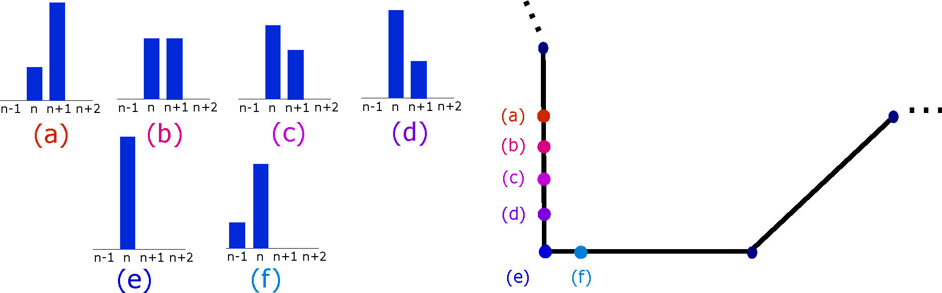
These states are equilibria to the unbiased equation because in each case, there is no one a distance 2 away from sites in the cluster to interact with. For sufficiently small bias, solutions trace out a path very close to this family of two-opinion clusters; the moving cluster stays concentrated on two sites as it shifts (see for example the simulations for small \(\beta\) above). For a smooth family of equilibria, one would seek to construct a slow manifold nearby. The family above, however, is not smooth - it possesses corners where the tangents are not continuous. We thus analyze the dynamics separately near the corners, combining this with analysis in between, to obtain asymptotic drift speeds for the clusters as \(\beta \to 0\): we find \(c\sim \frac{2\beta m}{\pi}\).
We are able to compare this with speeds obtained from numerical continuation (see below), and find agreement to leading order for small \(\beta\). However, the discrepancy for even moderately small values of \(\beta\) is significant. We conjecture that this discrepancy can be attributed to the passage near the one-site clusters, contributing a term \(\beta^{3/2}\).
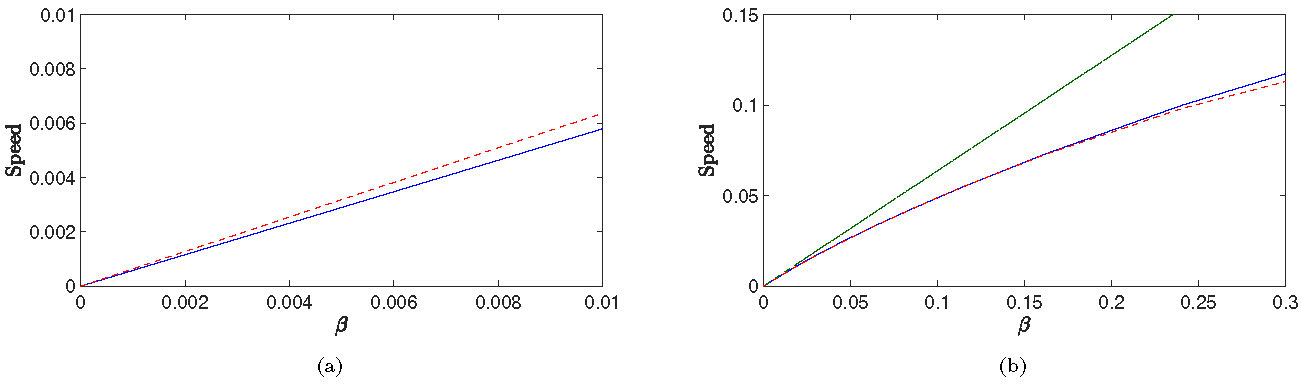
Figure 0.1: (a) Comparisons of leading order average drift speed prediction from theory (red) with drift speed from numerical continuation (blue) for a cluster of total mass 1. (b) Numerically computed values for the drift speed (blue) plotted against the leading-order approximation (green) and the approximation with the \(\beta^\frac{3}{2}\) correction.
Too much bias… breaks down consensus?!
The curious phenomenon from the simulations can be supported with a linear stability analysis, where we find that for \(\beta > 2\), the uniform state becomes (linearly) stable. One first considers the linearization of the equation at the uniform state \(P_n \equiv m\):
| |
\( \frac{dP_n}{dt} = m\left(-P_{n-2} + 2P_{n-1} -(2+2\beta)P_n + (2+2\beta)P_{n+1} - P_{n+2}\right). \) |
|
Inserting an ansatz $P_n=e^{i\sigma n + \lambda t}$, one can then find the relationship
| |
\( \lambda = m(-2\cos(2\sigma) + (4+2\beta)\cos(\sigma) -(2+2\beta) + 2i\beta\sin(\sigma)), \) |
(0.3) |
which relates the linear growth rate \(\lambda\) in time to the spatial frequency \(\sigma\) of a periodic perturbation.
For \(\beta \ge 2\), the real part of \(\lambda\) is nonpositive, leading to linear stability of the uniform state. Strong enough bias thus stabilizes the uniform distribution of opinions, and disfavors conensus!
The interested reader should at this point try to reconcile this to themself. Why should this be? Why would strong bias disfavor clustering? (The authors have some ideas, but it is perhaps more interesting to leave them to the end.)
Numerical Continuation
One can solve, numerically, for traveling-wave solutions directly, rather than simulating the the entire dynamics, by first formulating the problem as an equation \(F(P) = 0\), for some function \(F\). In order to do this, we write the opinion distribution in the form we want - a single shifting profile, \(P_n = Q(n + ct)\), where \(Q\) is now a real-valued function.
If this is difficult to visualize, the video above shows what a fixed profile (blue) looks like as it moves through the lattice points (red). This perhaps also recalls the direct simulations above, some of which resembled the red curves.
In the above format, the profile \(Q(x)\) satisfies the functional equation
| |
\( 0 = - c Q'(x) + 2 Q(x-1) Q(x+1) - Q(x) \big( Q(x-2) + Q(x+2) \big) + \beta \big( Q^2(x+1) - Q^2(x) \big). \) |
(0.4) |
This is an equation of the form \(F(Q) = 0\), which we would like to solve numerically. In order to do so, we:
We solve these \(N+2\) equations in the variables \((Q, c, \mu)\). We then add the variable \(\beta\) as a parameter, and use secant continuation, a form of numerical continuation, in order to track the family of solutions as \(\beta\) increases. Such methods rely on the fact that as the parameters are varied slowly, the previous solution can be used to inform the initial guess for the next iteration.
Nonlocal Taylor Series (or how to make a Calc 2 Student Angry)
We would also like to highlight a key ingredient in the proof of existence of traveling clusters in regime (iii). The method is perhaps most easily explained through example, so some detail follows.
If we seek to find traveling-wave solutions of the form \(m + q(x) = m + q(n+ct) = P_n(t)\) near \(\beta = 2\), we get the following equation, similar to the equation solved numerically above:
| |
\( 0 = -c q'(x) + m(2q(x -1) + 2(\beta + 1)q(x + 1) - 2(\beta + 1)q(x) - q(x -2) - q(x+2) + \mathcal{N}(q,\beta)), \) |
(0.5) |
where \(\mathcal{N}(q,\beta) = 2 q(x-1)q(x+1) - q(x) ( q(x-2) + q(x+2)) + \beta ( q(x+1)^2 - q(x)^2)\). This is an example of a forward-backward delay equation, since the value of \(q(x)\) depends on both the `future' \(q(x+1)\) and the `past' \(q(x-1)\). We can reframe this as a nonlocal equation (!), an equation involving a spatial convolution kernel, by writing \(q(x+1) = \delta(\cdot + 1)*q\), and repeating for each delay term to get an equation of the form
| |
\( 0 = -c q'(x) - 2m (\beta + 1) q(x) + m \mathcal{K}*q + \mathcal{N}(q,\beta), \) |
(0.6) |
with \(\mathcal{K}\) a sum of shifted Dirac deltas. With this, we are able to use recently developed methods [3, 9] for nonlocal equations to derive a center manifold expansion for (0.5).
Classically, to find center manifolds, one splits the phase space into a center subspace (the linear kernel, and the coordinate of interest) and a hyperbolic subspace (where there is linear decay or growth), and then one writes the manifold as a graph over the center subspace. Invariance is then used to find the Taylor coefficients of the graph. Here, too, we write
| |
\( q = q_0 + \Psi(q_0, \beta, c) \) |
(0.7) |
where \(q_0 = q_0(x) = A_0 + A_1 x + A_2 x\) is an element of the center subspace, or the kernel of the linear part of (0.6), \(\mathcal{T} q = -c q'(x) - 2m (\beta + 1) q(x) + m \mathcal{K}*q\). Note that we are considering \(q\) as an element of solution space, or function space. When we expand the graph \(\Psi\), we then expand in both the kernel basis elements \(A_0, A_1, A_2\), and the parameters \(\beta, c\):
| |
\( \Psi (A_0, A_1, A_2, \beta, c)= \sum_{\underset{|l|+|r|>1}{l, r}} \psi_{l,r}(x) A_0^{l_0} A_1^{l_1} A_2^{l_2} (2-\beta)^{r_1} (c-4)^{r_2}, \) |
(0.8) |
Here, the Taylor coefficients \(\psi_{l,r}\) we are looking for here are functions, because the hyperbolic subspace is a subset of function space.
Although this would make your Calculus 2 students deeply uncomfortable, it greatly simplifies computation. As in the finite-dimensional case, we plug the center manifold (0.7) into the differential equation, and at quadratic order we obtain:
| |
\( \mathcal{T}\left(\sum_{|l| + |r| = 2} A_0^{l_0} A_1^{l_1} A_2^{l_2} \tilde{\beta}^{r_1} \tilde{c}^{r_2} \psi_{l_0,l_1,l_2,r_1,r_2}(x) \right)
= 4 A_0A_1 + 4 x A_1^2 + 8 x A_0 A_2 + (12 x^2 + 4) A_1A_2 + (8 x^3 + 8 x + 4) A_2^2 \\ \qquad - 2m A_1 \tilde{\beta} - A_1 \tilde{c} + (-2m-4mx)A_2 \tilde{\beta} -2 x A_2 \tilde{c}, \) |
|
where \(\mathcal{T}\) is the linear part of (0.6). Because convolution preserves polynomials, we are able to insert polynomials \(c_3 x^3 + c_4 x^4 + c_5 x^5 + c_6 x^6\) as an ansatz for each \(\psi_{l,r}\), and then match coefficients, both in \(x\) and in \(A_0,A_1,A_2\). For instance, to find \(\psi_{(1,1,0),(0,0)}\), examining the coefficients of \(A_0 A_1\), we find
| |
\( (4m) c_3 + (16m x - 24m)c_4 + (40 m x^2 - 120m x +4m) c_5 + (80x^3-360m x^2+24m x -120m) c_6 = 4. \) |
|
We thus get \(c_3 = -\frac{1}{m}\), and \(\psi_{(1,1,0),(0,0)} = \frac{-1}{m}x^3\). The rest of the computations of \(\psi_{l,r}\) follow similarly, if a bit more tediously, and as a note, it is recommended to employ a large number of second opinions or ideally a computer to check one's arithmetic.
Lastly, in order to calculate a reduced vector field from the center manifold, as in the finite-dimensional case, one 1) considers the flow on the center manifold, 2) projects it down to the center subspace, and then 3) differentiates the projected flow at time 0.
The reason for expanding in the space of functions as we did is that for a nonlocal equation, one doesn't have a flow or vector field in phase space (or even a phase space) - but in the space of functions, one does. In solution space, the time-\(t\) flow is the action that takes \(q(x)\) to \(q(x + t)\). We can therefore calculate
| |
\( q_0' = \frac{d}{d t} \mathcal{P}\left((q_0 + \Psi)(x + t)\right)\Big|_{t = 0}. \) |
(0.9) |
combining steps 1)-3) together, using the projection \(\mathcal{P} (q) = q_0 + q'(0) x + \frac{1}{2} q''(0) x^2\). This yields a three-dimensional system of ordinary differential equations in \(A_0, A_1, A_2,\) which reduces to a third-order equation, and can be further reduced to the second-order equation
| |
\( 0 = a_0'' -a_0 + a_0^2 -\tilde{\beta}^\frac{1}{2}\sqrt{3} \left[3(1+\frac{c_0}{2})^\frac{1}{2} a_0a_0'-(1+\frac{c_0}{2})^{-\frac{1}{2}}(2+\frac{3c_0}{4})a_0' \right] + \mathcal{O}(\tilde{\beta}) \) |
(0.10) |
after using a conserved quantity, related to population conservation in the original equation.
One must still show that (0.10) has a family of solutions of the kind we desire - but one can. The focus of this section is that the nonlocal center manifold expansion allows us to reduce the infinite-dimensional system to one second-order equation, which one can analyze using more standard Melnikov methods (which we omit here).
I hope you are left with more questions than answers after reading this. If anything, one should feel that studying social dynamics is valuable from a large variety of viewpoints (interested readers should also check out the AMS Special Session on Complex Social Systems at JMM 2024), even within the field of mathematics.
Olivia Cannon delivered a minisymposium presentation on this research at the 2023 SIAM Conference on Applications of Dynamical Systems, which took place in Portland, Oregon, earlier this year. This work can also be found as a recent arXiv preprint: https://arxiv.org/abs/2302.04214.
References
[1] E. Ben-Naim, Opinion dynamics: Rise and fall of political parties, Europhysics Letters (EPL), 69(5), 2005, pp. 671-677.
[2] O. Cannon, T. Bondurant, M. Whyte, and A. Scheel, Shifting consensus in a biased compromise model, 2023.
[3] O. Cannon and A. Scheel, Coherent structures in nonlocal systems - functional analytic tools, 2023.
[4] T. Carletti, D. Fanelli, S. Grolli, and A. Guarino, How to make an efficient propaganda, EPL (Europhysics Letters), 74:222, 01 2007.
[5] S. Chen, D. H. Glass, and M. McCartney, Characteristics of successful opinion leaders in a bounded confidence model, Phys. A, 449(C), 2016, pp. 426-436.
[6] G. Deffuant, D. Neau, F. Amblard, and G. Weisbuch, Mixing beliefs among interacting agents, Advances in Complex Systems, 3(01n04), 2000, pp. 87-98.
[7] M. Del Vicario, A. Scala, G. Caldarelli, H. Stanley, and W. Quattrociocchi, Modeling confirmation bias and polarization, Scientific Reports, 7, 06 2016.
[8] I. Douven and R. Hegselmann, Mis- and disinformation in a bounded confidence model, Artificial Intelligence, 291, 11 2020.
[9] G. Faye and A. Scheel, Center manifolds without a phase space, Trans. Amer. Math. Soc., 370(8), 2018, pp. 5843-5885.
[10] W. Han, C. Huang, and J. Yang, Opinion clusters in a modified hegselmann–krause model with heterogeneous bounded confidences and stubbornness, Phys. A, 531:121791, 2019.
[11] R. Hegselmann and U. Krause, Opinion dynamics and bounded confidence models, analysis and simulation, Journal of Artificial Societies and Social Simulation, 5, 07 2002.
[12] J. Kertesz, A. Sirbu, F. Gianotti, and D. Pedreschi, Algorithmic bias amplifies opinion polarization: A bounded confidence model, in StatPhys 27 Main Conference, 2019.
[13] J.-D. Mathias, S. Huet, and G. Deffuant, Bounded confidence model with fixed uncertainties and extremists: The
opinions can keep fluctuating indefinitely, J. Art. Soc. and Soc. Sim., 19(1):6, 2016.
[14] W. Quattrociocchi, G. Caldarelli, and A. Scala, Opinion dynamics on interacting networks: media competition and social influence, Scientific Reports, 4, 2014.
[15] D. Shen and Z. Sun, Finite-time convergence of kh model under asymmetric confidence levels, in 2009 IEEE International Conference on Control and Automation, 2009, pp. 224-227.