I’m a postdoctoral research fellow at The Mathematical Biosciences Institute (MBI) with research interests in parabolic partial differential equations and multi-scale techniques (e.g., homogenization), especially applied to problems motivated by biology. For fruitful interaction with biologists, you need numerical experiments as well as theoretical results, and so I also implement these models by finite element method and increasingly analyze them using statistical frameworks for global sensitivity and Bayesian inference.

1. Concentrated capacity for protein dynamics

In a recent single author work [1], I have proposed a novel and multi-scale partial differential equations model inspired by solvent interacting with protein at the molecular scale. Proteins are chains of amino acids linked together in sequence along a polypeptide bond and are the molecular machines that drive many dynamics inside biological cells. In molecular dynamics (MD) simulations [2, 3], resolving the motion of the explicit solvent which surrounds the protein is a great computational expense [2, Sec 8.3]. However, the localized interaction of solvent at different sites along the protein can strongly influence the conformation the protein takes [4, 5], which in turn affects its ability to bind its targets or otherwise properly function. Owing to the chain-like nature of its primary sequence structure along covalent bonds, here a protein is modeled as an intrinsically 1d object in 3d space which advects its surrounding solvent at their exact point of contact.

The key analytical technique I introduce to this problem is the so-called concentrating capacity [6, 7, 8], which like homogenization, accommodates the presence of multiple physical scales. However, unlike the latter which averages the small scales into the larger, this technique resolves the small scale dynamics onto their intrinsic lower dimension. In particular, the technique is shown to make precise a parabolic PDE whose equations coefficients are highly singular, time-varying measures.

Concentrating capacity is performed over a family of diffusion-advection equations whose advection velocities weakly approximate a Dirac-mass at a moving curve \(\vec{v}_C(t;x)d\delta_{\Gamma(t)}/d\mu_{\mathrm{Leb}}\). Here \(\Gamma(t)\) is the moving curve within the domain \(\Omega\)'s interior. Crucially, as stated this family lacks the compactness necessary to justify a limit. Concentrating capacity remedies this difficulty by not only introducing Dirac-mass approximations in advection but aggregating them into the time derivative and diffusion terms as well. This leads to the family of diffusion advection equations, indexed by \(\epsilon\),\(\delta\),

\( \partial_t\left[a_{\epsilon,\delta}(t;x)u_{\epsilon,\delta}\right] + \mathrm{div}\left[-\mathbb{K}_{\epsilon,\delta}(t;x)\nabla u_{\epsilon,\delta} + u_{\epsilon,\delta}\vec{v}_{\epsilon,\delta}(t;x)\right] = 0. \)

The coefficient weights are of order \(O(\epsilon^{-2})\) about the curve to limit towards the Dirac-mass. The \(\delta\) approximation is needed for a time-differentiable transition between behaviors in bulk and about the curve.

A weak solution is extracted by taking \(\epsilon,\delta(\epsilon)\rightarrow 0\) and characterized by a novel (i.e., concentrated capacity) diffusion law. The limit characterizes a system for the pair \((\mathfrak{u},\mathfrak{u}_C)\) quantifying concentration of solvent in the volume and concentration localized at the curve respectively. From the weak form, we may extract formal, pointwise limits in the volume and at the curve with novel components. Note \(k_s\), \(k_n\) are diffusion coefficents along tangential and normal curve directions while \(k_0\) is the diffusion coefficient for bulk:

• The limit in the volume:

\( \partial_t\mathfrak{u} - k_0\Delta\mathfrak{u} = 0 \mbox{ in } \Omega\setminus \Gamma(t) \)

• The limit at the curve:

\( \partial_t\left(\mathfrak{u}_C\frac{d\delta_{\Gamma(t)}}{d\mu_{\mathrm{Leb}}}\right) - \mathrm{div}\left(\mathcal{K}\nabla\mathfrak{u}_C\frac{d\delta_{\Gamma(t)}}{d\mu_{\mathrm{Leb}}}\right)+ \mathrm{div}\left(\mathfrak{u}_C\vec{v}_C\frac{d\delta_{\Gamma(t)}}{d\mu_{\mathrm{Leb}}}\right) \)

\( = \left(\frac{1}{\pi\epsilon^2_0}\lim_{\epsilon\rightarrow 0}\int_{\mathcal{D}_\epsilon(\Gamma)}k_0\Delta\mathfrak{u}\right)\frac{d\delta_{\Gamma(t)}}{d\mu_{\mathrm{Leb}}} \mbox{ on } \Gamma(t) \)

- The limit for \(\mathfrak{u}_C\) is coupled to \(\mathfrak{u}\) by the distributional \(\Delta \mathfrak{u}\) on the right-hand side. An infinitesimal local flux about the curve, integrated over cross-sections and coming from the volume, acts as a source term along the curve length.

- In local coordinates, there is a diffusion-advection instantaneously in the arc-length parameter, \(s\), of the curve. Advection is the tangential projection along \(\Gamma\), \(\vec{t}\), of the slip between the prescribed, local advection and the curve motion:

\( \partial_t\mathfrak{u}_C + \partial_s\left[-k_s(s)\partial_s\mathfrak{u}_C + \mathfrak{u}_C\left(\vec{t}\cdot\left(\vec{v}_C(t;s) - \dot{\Gamma}(t;s)\right)\right)\right] \)

- Since \(\mathfrak{u}_C\) is defined along \(\Gamma(t)\), differentiating along normal directions is not defined. Nevertheless, the limiting process retains a memory of the orthogonal gradient in a weak sense. In particular, slip between the local advection flow and curve motion (de)compresses localized material which diffusion acts to relieve:

\( \nabla_{\bot}\mathfrak{u}_C = \mathrm{proj}_{\left\langle \vec{t}\right\rangle^{\bot}}\left(\vec{v}_C - \dot{\Gamma}\right)\mathfrak{u}_C/k_n(s) \)

- If the expression for the weak orthogonal gradient is substituted into the limit, and \(\nabla\mathfrak{u}_C\) is reinterpreted for \(\mathfrak{u}_C\) with its constant extension into the volume, then it is seen that the new effective advection velocity, \(\vec{v}_{C,\mathrm{eff}}\), is not simply the prescribed \(\vec{v}_{C}\). Only the tangential component survives while the normal components become that of the curve's own motion:

\( \vec{v}_{C,\mathrm{eff}} = \mathrm{proj}_{\vec{t}}\;\vec{v}_C + \mathrm{proj}_{\left\langle \vec{t}\right\rangle^{\bot}}\;\partial_t\Gamma \)

• The global limit:

\( \partial_t\left(\mathfrak{u}+\pi\epsilon^2_0\mathfrak{u}_C\frac{d\delta_{\Gamma(t)}}{d\mu_{\mathrm{Leb}}} \right) - \mathrm{div}\left(k_0\nabla\mathfrak{u} + \pi\epsilon^2_0\mathcal{K}\nabla\mathfrak{u}_C\frac{d\delta_{\Gamma(t)}}{d\mu_{\mathrm{Leb}}} \right) + \mathrm{div}\left(\pi\epsilon^2_0\mathfrak{u}_C\vec{v}_C\frac{d\delta_{\Gamma(t)}}{d\mu_{\mathrm{Leb}}} \right) \)

\( =0\mbox{ in } \Omega \)

- While \(\Gamma(t)\) is 1d, the limit retains a memory of the original cross-sectional area \(\pi\epsilon^2_0\), before the concentrated capacity limit was performed. For simplicity this work assumed discal cross-sections, but the technique can be applied to general, even space-varying, cases.

- The same considerations as for the limit at the curve apply.

While an idealized model for an application that is accustomed to very fine detail, nonetheless, this project is an example of how novel mathematics may be inspired by biology, and it remains to be seen how far this approach may be pushed. The aspiration would be to develop a PDE's model of 3d protein-solvent interactions with the computational expense of an essentially 1d problem. Future tests for this framework include quantifying solution regularity and numerical implementation, the addition of amino-acid sidechains, and coupling to protein motion as well as multiphysics phenomena such as dielectric effects. Beyond the direct use of molecular force-fields, the concentrated capacity limit opens up the possibility of functionals built from local solvent concentration with variational, gradient-flow frameworks for encoding hydrophobic and hydrophilic protein regions.

2. Homogenization and parameter sensitivity for visual transuction

I was introduced to homogenization and concentrated capacity in a project applied to rod and cone photoreceptors in vision [10, 11, 12]. In Fig 2, a cone photoreceptor is rendered by a finite element mesh except in actual simulations the number of chambers (green conical cuts) is 30-50x's larger. Homogenization used a limiting process over a family of approximating PDE's to express the small-scale geometric contributions (e.g., chambers) by a novel PDE law whose numerical implementation is much more efficient compared to a standard diffusion model set to the original geometry.

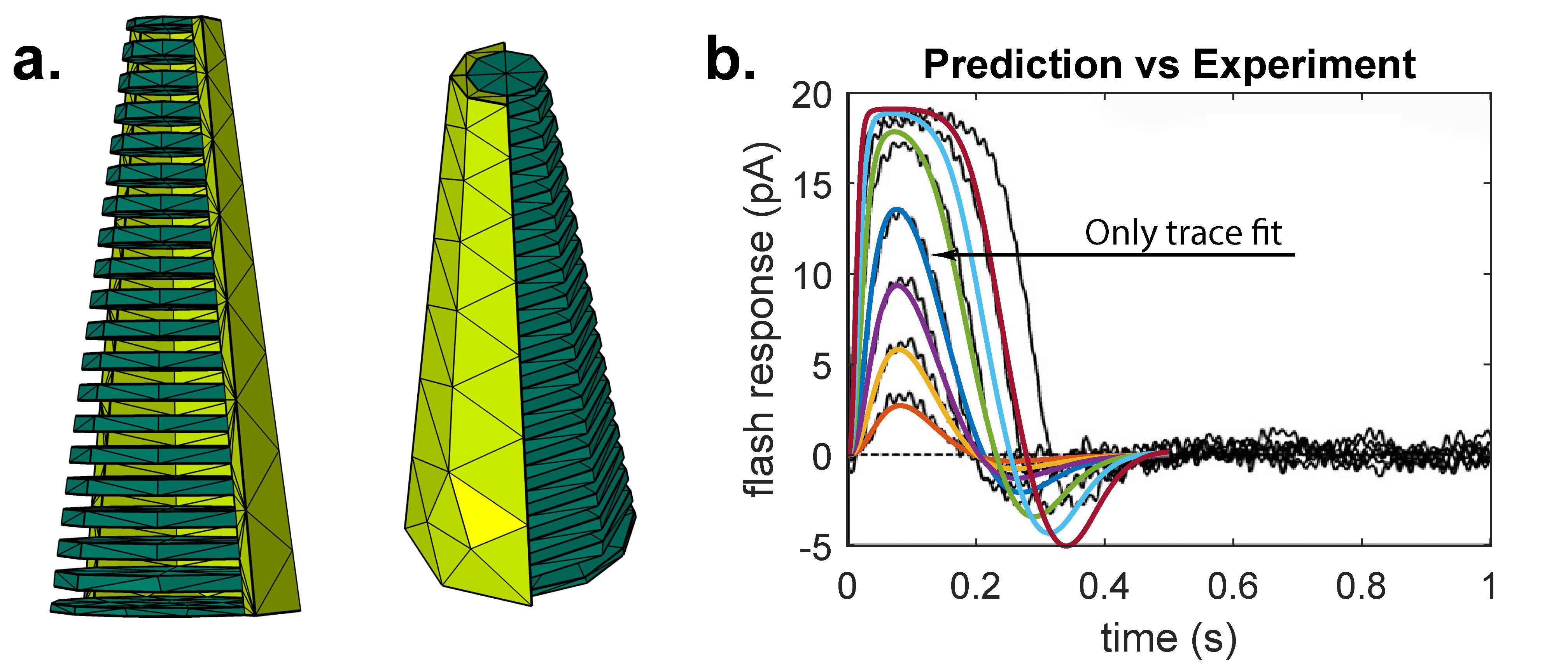
Figure 2. (a.) Illustrative, coarse finite element mesh for a cone photoreceptor, before homogenization, with artificially low number of diffusion chambers. Actual number of chambers is 300-500. (b.) Experimental traces (black) of striped bass cone recording [9] compared to model prediction (colored traces). MCMC optimizes model parameters while satisfying known constrains on output. Model reproduces experiment even for traces not fit with some deviation at saturating light intensity.

Since that time, this project has grown to experimental prediction and parameter sensitivity analysis alongside experimental collaborators in the Vanderbilt Pharmacology Department and Boston University School of Medicine. In a soon to be submitted work, I have introduced Markov Chain Monte Carlo explorations of parameter space to optimize model parameters while satisfying known experimental constraints even where these constraints are not made on free parameters. I have also introduced Sobol indices [13, 14] to the project for global sensitivity analysis based on experimental parameter ranges reported in the literature. Sobol indices quantify the percentage of model variance attributed to interactions between a freely selected subset of model parameters through an orthogonal decomposition made rigorous in the topology of \(L^2\). A noteworthy finding indicates that photoreceptor geometry at the nm scale may contribute to \(\sim\) 50% of the variance in flash response even though gross morphology at the \(\mu m\) scale has been evidenced as less significant experimentally [15].

References

[1]   C. Klaus, A concentrated capacity model for diffusion-advection: advection localized to a moving curve, 2020, https://arxiv.org/abs/2010.14789.

[2]   S. A. Adcock and J. A. McCammon, Molecular dynamics: survey of methods for simulating the activity of proteins, Chem. Rev., 106(5), pp. 1589-1615, May 2006.

[3]   R. O. Dror, R. M. Dirks, J. P. Grossman, H. Xu, and D. E. Shaw, Biomolecular simulation: a computational microscope for molecular biology, Annu. Rev. Biophys., 41, pp. 429-452, 2012.

[4]   M. C. Bellissent-Funel, A. Hassanali, M. Havenith, R. Henchman, P. Pohl, F. Sterpone, D. van der Spoel, Y. Xu, and A. E. Garcia, Water determines the structure and dynamics of proteins, Chem. Rev., 116(13), pp. 7673-7697, July 2016.

[5]   D. Laage, T. Elsaesser, and J. T. Hynes, Water Dynamics in the Hydration Shells of Biomolecules, Chem. Rev., 117(16), pp. 10694-10725, Aug 2017.

[6]   P. Colli and J. F. Rodrigues, Diffusion through thin layers with high specific heat, Asymptotic Anal., 3(3), pp. 249-263, 1990.

[7]   E. Magenes, Stefan problems in a concentrated capacity, In Advanced mathematics: computations and applications, NCC Publ., Novosibirsk, pp. 82-90, 1995.

[8]   L. Gioia and A. Keller, Homogenization and concentrated capacity for the heat equation with two kinds of microstructures: uniform cases, Ann. Mat. Pura Appl. (4), 196(3), pp. 791-818, 2017.

[9]   J. I. Korenbrot, Speed, sensitivity, and stability of the light response in rod and cone photoreceptors: Facts and models, Prog. Retin. Eye Res., 31, pp. 442-466, 2012.

[10]   C. Klaus, G. Caruso, V. V. Gurevich, and E. DiBenedetto, Multi-scale numerical modeling of spatio-temporal signaling in cone phototransduction, PLoS ONE, 14(7), p. e0219848, https://doi.org/10.1371/journal.pone.0225948.

[11]   C. Klaus and G Caruso, Finite element package for cone visual transduction, Zenodo, Feb 2019, https://doi.org/10.5281/zenodo.2561347.

[12]   G. Caruso, V. V. Gurevich, C. Klaus, H. Hamm, C. L. Makino, and E. DiBenedetto, Local, nonlinear effects of cGMP and Ca2+ reduce single photon response variability in retinal rods, PLoS One, 14(12), p. e0225948, 2019, https://doi.org/10.1371/journal.pone.0225948.

[13]   I. M. Sobol, Global sensitivity indices for nonlinear mathematical models and their Monte Carlo estimates, Math. Comput. Simulation, 55(1-3), pp. 271-280, 2001. The Second IMACS Seminar on Monte Carlo Methods (Varna, 1999).

[14]   A. Saltelli, P. Annoni, I. Azzini, F. Campolongo, M. Ratto, and S. Tarantola, Variance based sensitivity analysis of model output. Design and estimator for the total sensitivity index, Comput. Phys. Comm., 181(2), pp. 259-270, 2010.

[15]   A. Morshedian and G. L. Fain, Single-photon sensitivity of lamprey rods with cone-like outer segments, Curr. Biol., 25(4), pp. 484-487, Feb 2015.