Christian Hamster and Peter van Heijster, Wageningen University and Research.

The results in this article are a summary of those in Christian Hamster and Peter van Heijster, Waves in a stochastic cell motility model, Bulletin of Mathematical Biology, 85(8):70, 2023.

Introduction

In order to move around, an amoeboid cell can change its shape by polymerizing actin to curve the cell membrane. The actin polymerization is controlled by signaling molecules and experiments have shown that activation of these signaling molecules happens at localized patches that can move along the cell membrane like a wave [1, 13]. In wild-type (WT) cells, these waves move fast and die out, creating healthy-shaped pseudopods, while in cancerous cells these waves can stick to a point, creating elongated protrusions [1], see Figure 1.

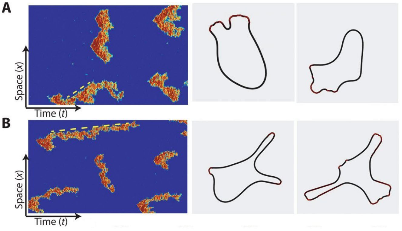
Figure 1: Stochastic simulations of the microscopic Gillespie-type model from [1]. The figures on the left show stochastic simulations of the Ras activity for parameter values applicable to (A) wild-type cells and to (B) genetically modified cells, where the phosphatase PTEN has been switched off. The figures on the right show typical cell shapes corresponding to the dynamics in the left figures. This shows that mutations in the gene that codes for PTEN lead to elongated protrusions typically associated with cancer. The dotted yellow line is an indicator of the wave speed, i.e. the actin waves in (B) are slower and live longer than in (A). Reproduced from [1] under creative commons license 4.0.

Without an external signal, the formation of these pseudopods happens at random places on the cell membrane, resulting in random motion. In contrast, when a cell senses a chemical signal, it can concentrate the random protrusions at the side of the cell where the signal comes from, leading to movement in the direction of the signal [4]. This implies that an external signal does not necessarily activate the dynamics at a certain point on the membrane, but rather changes the random walk of the cell into a biased random walk in the direction of the signal. As cells are small, the difference in signal strength between the front and the back of the cell (the gradient) is small as well. Therefore, an important question in cell biology is "How can a cell use a small gradient in the signal to concentrate the actin activity in the front?". This question has been studied intensively over the past decades, see [5] for a review.

How do we translate the problem described here into a mathematical framework? Generally, two options are used. First, there is a Gillespie-type algorithm [8, 9] which can be used successfully to simulate the involved chemical reactions on a microscopic level, as shown in Figure 1. For individual molecules, the probabilities of diffusing from one grid cell to another, or taking part in a chemical reaction, are prescribed. Note that this description is highly stochastic and computationally very expensive. Furthermore, this approach is difficult to analyze mathematically. A second option, that will be familiar to most of us, is to use the chemical reactions to derive a large-scale macroscopic equation. Instead of individual molecules in grid cells, we assume densities of molecules on a continuous domain, described by a reaction-rate equation with diffusion, also known as a Reaction-Diffusion Equation (RDE). Now, when we simulate this RDE with the same parameters as in Figure 1, we run into a problem. As Figure 2 shows, for both sets of parameters, there are counterpropagating traveling waves. These simulations are not only visually very different from Figure 1, but the parameter change in the RDE does qualitatively change the solution. This then implies that the RDE is not a useful tool to study these chemical reactions. To solve this issue, we need to take a step back in the modeling process.

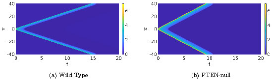
Figure 2: Two simulations of PDE (1) with parameters as in [1]; \(D_u=0.1\), \(a_1=0.167\), \(a_2=16.67\), \(a_4=1.44\), \(a_5=1.47\), \(D_v=1\), \(\varepsilon=0.4\), \(c_1=0.1\) and, for Figure (a), \(a_3=167\) and \(c_2=2.1\), while \(a_3=300.6\) and \(c_2=3\) for Figure (b). The initial condition is a bump with the shape of \(1/\cosh(\cdot)\).

Modeling

In [1], the choice is made to describe the highly complex actin dynamics with a conceptual activator \(u\) and inhibitor \(v\) that diffuse and react with each other. The species \(u\) and \(v\) are an abstraction of the dozens of components that regulate the actual cell movement. Using a Gillespie algorithm, activation events that resemble those of healthy and cancerous cells can be recreated, see Figure 1. In the macroscopic limit, the stochastic model is reduced to an RDE:

\( \begin{split} \partial_t u&=D_u \partial_{xx} u -a_1 u-a_2uv+\frac{a_3u^2}{a_4+u^2}+a_5\,,\\ \partial_t v&=D_v \partial_{xx} v +\varepsilon(-c_1v+c_2u), \end{split} \)

(1)

which is the RDE we simulated in Figure 2. This model is a variation on the classic FitzHugh-Nagumo model for neuron spiking [7, 15]. From the figures, it is clear that there is a significant difference between the dynamics of the two approaches.

It is important to realize that the dynamics of the different chemical processes in the cell are inherently stochastic and at the size of a single cell, chemical reactions are not well approximated by large-scale approximations. In other words, treating the relevant enzymes and receptors like a continuous medium of infinitely many, infinitely small, particles is invalid, and the stochastic nature of reactions between individual molecules becomes essential.

In between the macroscopic level of the RDE and the microscopic level of the chemical reactions, one can derive a mesoscopic Stochastic PDE, known as a Chemical Langevin Equation (CLE) [10]. Without going into too much detail here, the derivation of the CLE is based on the following idea. Suppose we have a grid cell with a number of molecules \(N(t)\) and a chemical reaction that creates new molecules with propensity \(a(N(t))\), meaning that the time we have to wait for a new molecule to be created is exponentially distributed with parameter \(a(N(t))\). When enough reactions occur in the interval \([t,t+dt]\), we assume that \(N(t+dt)\) is well approximated by \(N(t+dt)=N(t)+dt\mathcal{P}(a(N(t)))\), where \(\mathcal{P}\) is a Poisson distribution. Next, we define a density \(x(t)=N(t)/\Omega\) and the discrete Poisson distribution is approximated by a continuous Gaussian with average and variance \(a(N(t))\) (again assuming \(N(t)\) is large enough), resulting in \(x(t+dt)=x(t)+a(x(t))dt+\frac{\sqrt{dt}}{\sqrt{\Omega}}\sqrt{a(x(t))}\xi\), where \(\xi\) is drawn from \(\mathcal{N}(0,1)\). \(\Omega\) is here the "scale" or volume of the system. Upon taking the limit of \(dt\to0\), we arrive at a Stochastic Differential Equation (SDE):

\( dx(t)=a(x(t))dt+\frac{1}{\sqrt{\Omega}}\sqrt{a(x(t))}d\beta_t, \)

(2)

with \(\beta_t\) a Brownian motion. However, note that the derivation above only makes sense for "intermediate" values of \(dt\). When \(dt\) is too small, there are not enough reactions to approximate a Poisson distribution, but when \(dt\) is too large, we cannot use \(a(N(t))\) to describe the propensity in the interval \([t,t+dt]\). For a more detailed explanation, see [3]. For readers familiar with system size expansion (or van Kampen's Expansion) of chemical master equations [16], note that the Fokker-Planck equation of this SDE is identical to the Fokker-Planck equation found in the system size expansion.

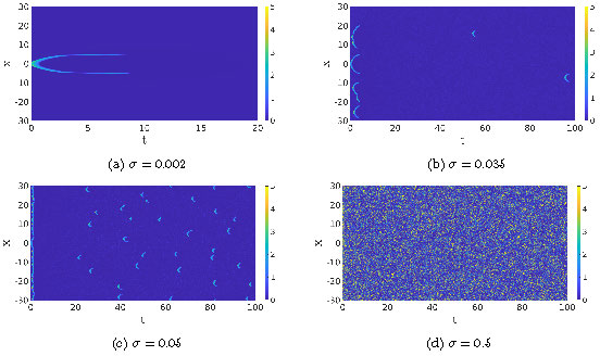
Figure 3: The \(u\)-component of the SPDE (3) for four different values of the noise \(\sigma\). In Figure (a), we only show the simulation of wave integrated up to \(T=20\) because the solution remains in the background state afterward, the other three figures are shown up to \(T=100\).

When we add in a stochastic diffusion equation, we end up with the following SPDE:

\( du =\left(D_u \partial_{xx} u-(a_1+a_2v)u+\frac{a_3u^2}{a_4+u^2}+a_5\right)dt\\ \qquad\qquad+\sigma\sqrt{(a_1+a_2v)u+\frac{a_3u^2}{a_4+u^2}+a_5}\,dW^1_t +\sigma\partial_x\left(\sqrt{2D_uu}\,d\tilde W^1_t\right),\\ dv =\left(D_v \partial_{xx}v+\varepsilon(-c_1v+c_2u)\right)dt\\ \qquad\qquad+\sigma\sqrt{\varepsilon(-c_1v+c_2u)}\,dW^2_t+\sigma\partial_x\left(\sqrt{2D_vv}\,d\tilde W^2_t\right). \)

(3)

The square root terms come from variations in the chemical reactions, as described above, while the \(\partial_x\sqrt{\cdot}\) term comes from the stochastic diffusion equation [6]. Here, \((d W^{1}_t, d W^{2}_t)\) and \((d \tilde{W}^{1}_t,d \tilde{W}^{2}_t)\) are two independent noise vectors with space-time white noise (each component is also independent of the other) and \(\sigma\) is a measure for the strength of the noise. Indeed, in the no-noise limit \(\sigma \to 0\) the mesoscopic SPDE (3) reduces to the macroscopic RDE (1). In that sense, \(\sigma\) serves as a scale parameter. This becomes clear from Figure 3. In these four simulations, we set the same initial condition. For large-scale simulations, i.e. \(\sigma\) small, we see that the deterministic pattern dominates (a double pulse), but subsequently gets destroyed and does not reappear again. For small-scale simulations, i.e. high values of \(\sigma\), there is no observable pattern. Only at intermediate scales, do we see activation events resembling the dynamics in Figure 1. Especially, we see that the background state can be activated by the noise.

When we compare the deterministic simulation with the stochastic simulation, there is a clear difference. The main advantage of the SPDE description is, on one hand, that the solutions still show the rich dynamics of the Gillespie models, i.e. the activation and destruction of waves, but are computationally significantly less expensive. On the other hand, since the SPDE in the no-noise limit reduces to the deterministic RDE model (1), we can use well-developed Partial Differential Equation (PDE) theory to gain insight into the dynamics of the RDE (1) and use this to study the closely related SPDE, see for instance [11, 14]. To give an idea of the differences between the deterministic and stochastic models we plot two simulations in Figure 4. It is clear that the simulation of the SPDE paints a much more dynamic picture than the deterministic one, which is more in line with the inherently noisy nature of the cell's chemical processes. Hence, SPDEs are an invaluable tool in unraveling the dynamics of a cell.

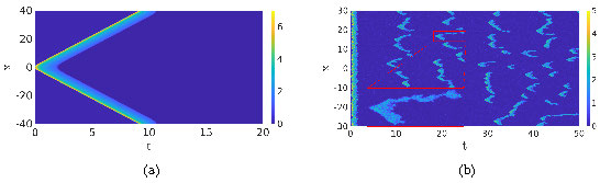
Figure 4: Comparison of the deterministic model (1) and its stochastic counterpart (3). In Figure (a) we show a simulation of (1), which is excited at \(t=0\), resulting in two counterpropagating traveling waves. In the stochastic simulation in Figure (b), the influence of the initial excitation quickly disappears and new pulses appear constantly. The same parameters are used as in the simulations shown in the second row of Figure 1. Observe the similarities in the shape of the activation events. In Figure (a), the two counterpropagating waves travel around the cell where they cancel each other, while in Figure (b) the waves cancel each other at a much shorter scale.

Wild-Type versus PTEN-null Cells

Now that we have an SPDE, we can again compare the model for the WT cells and the PTEN-null cells. In Figure 5, we compare the SPDE simulations of (3) to the Gillespie simulations from [1]. Focusing on the typical shape of the excitations, there is a clear qualitative correspondence between the two types of simulation. Furthermore, in both types of simulation, the average pulse duration is longer in the case of the PTEN-null cell simulations. Note that we show the SPDE simulations on a larger spatio-temporal scale to get a better idea of the distribution in shapes and the zoom-boxes highlight the detailed structure of a typical single activation event. In the case of PTEN-null cells, the background state can be excited for much lower noise values (\(\sigma\approx0.007\)), while for WT cells, the noise needs to be twice as large (\(\sigma\approx0.014\)) as a result of the increased values of \(c_2\) and \(a_3\). Hence, in PTEN-null cells, an already existing pattern can more easily sustain itself, leading to the elongated shapes of Figure 5(d).

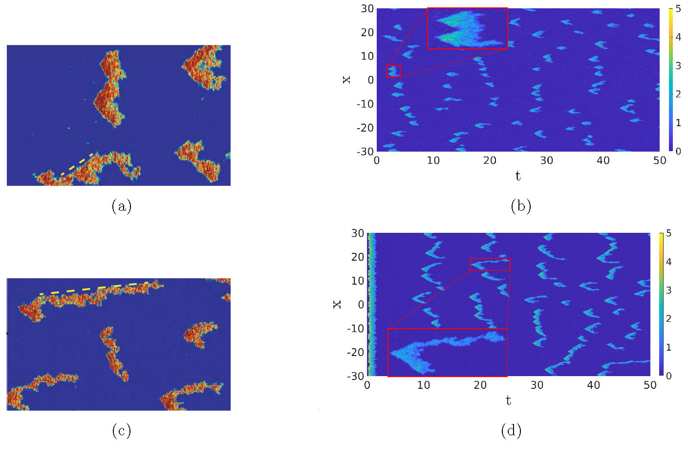
Figure 5: Comparison of the Gillespie model, Figures (a) and (c) from [1], versus the CLE approximation (3), Figures (b) and (d). The same parameters as in Figure 2, with \(\sigma=0.06\). The initial condition is \((u^*,2v^*)\). This can lead to an immediate excitation of the background state in Figure (d), while in Figure (b), the excitation of the background is more spread out. The zoom-boxes highlight the details of a single excitation.

The CLE and ad hoc approximations

The observation that the PDE and Gillespie simulations do not agree very well has been made before and in the literature ad hoc approaches to turn (1) into an SPDE can be found [1]. We are now also in the position to compare the CLE approach with the more ad hoc approach of adding additive space-time white noise to the \(u\)-component of (1) to mimic the inherent noisiness of the system. As is clear from Figure 1, not all activation events are equal, there is a significant variation in the length (or duration) of the events. When we run the simulation of the CLE a 100 times and determine for each observed event the length, we get a histogram as in Figure 6(a). When we run the same experiment with just white noise on the \(u\)-component, we find a histogram as in Figure 6(b). Note that the spread in length of the activation event is much larger in the CLE than with the white noise. Also, with just white noise, the activation events are all short and narrow and do not reflect the complicated dynamics of the underlying chemical reactions and experiments.

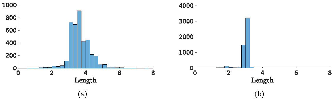
Figure 6: Figure (a) shows the histograms for the length of the activation events. In Figure (b), we again show the same histograms, but with just white noise on the \(u\)-component of (1). In order to compare the noise levels, we did not choose the same \(\sigma\) value for the two cases but chose \(\sigma\) values such that the average number of activation events per simulation is approximately 50.

Discussion & Conclusion

We have shown for a conceptual model as introduced in [1] that the CLE approach allows us to study the different possible patterns with relative ease, both qualitative and quantitative while remaining close to the underlying chemical processes. To understand differences in cell behavior, like the difference between wild-type and cancerous cells, the study of the statistical properties of the observed dynamics is essential. A natural question to ask is if all the stochastic terms introduced in the CLE (3) are really necessary. Could we, for example, ignore the noise term coming from the diffusion or forget the derivation of the CLE altogether and just naively add an additive white noise term to the equation for \(u\)? The histograms in Figure 6 indicate that additive noise does not recreate the rich structure of the chemical reactions. More simulations in [12] indicate that the effects of the terms that come from the diffusion are minimal (the \(\partial_x\sqrt{\cdot}\) term) and therefore can be ignored, making both simulations and analytical approaches easier.

In this paper, we studied a basic activator-inhibitor system with only a limited number of chemical reactions. However, the derivation of the CLE (3) holds for any number of molecules and for any number of chemical reactions. As such, one can see results described here as a proof of concept and the methodology of this paper can be directly applied to more complex regulating systems, such as the eight-component system designed in [2].

References

[1]   Sayak Bhattacharya, Tatsat Banerjee, Yuchuan Miao, Huiwang Zhan, Peter N. Devreotes, and Pablo A. Iglesias, Traveling and standing waves mediate pattern formation in cellular protrusions, Science Advances, 6(32):eaay7682, 2020.

[2]   Debojyoti Biswas, Sayak Bhattacharya, and Pablo A. Iglesias, Enhanced chemotaxis through spatially regulated absolute concentration robustness, International Journal of Robust and Nonlinear Control, 2022.

[3]   Paul C. Bressloff, Stochastic Processes in Cell Biology, volume 41, Springer, New York, 2014.

[4]   Youyuan Deng and Herbert Levine, Introduction to models of cell motility, In Karstan B. Blagoev and Herbert Levine, editors, Physics of Molecular and Cellular Processes, chapter 7, Springer, New York, 2022, pp. 173-212.

[5]   Peter N. Devreotes, Sayak Bhattacharya, Marc Edwards, Pablo A. Iglesias, Thomas Lampert, and Yuchuan Miao, Excitable signal transduction networks in directed cell migration, Annual Review of Cell and Developmental Biology, 33, 2017, pp. 103-125.

[6]   Elife Dogan and Edward J. Allen, Derivation of stochastic partial differential equations for reaction-diffusion processes, Stochastic Analysis and Applications, 29(3), 2011, pp. 424-443.

[7]   Richard FitzHugh, Impulses and physiological states in theoretical models of nerve membrane, Biophysical Journal, 1(6), 1961, pp. 445-466.

[8]   Daniel T. Gillespie, A general method for numerically simulating the stochastic time evolution of coupled chemical reactions, Journal of Computational Physics, 22(4), 1976, pp. 403-434.

[9]   Daniel T. Gillespie, Exact stochastic simulation of coupled chemical reactions, The journal of Physical Chemistry, 81(25), 1977, pp. 2340-2361.

[10]   Daniel T. Gillespie, The chemical langevin equation, The Journal of Chemical Physics, 113(1), 2000, pp. 297-306.

[11]   C. H. S. Hamster and Hermen Jan Hupkes, Travelling waves for reaction-diffusion equations forced by translation invariant noise, Physica D: Nonlinear Phenomena, 401:132233, 2020.

[12]   Christian Hamster and Peter van Heijster, Waves in a stochastic cell motility model, Bulletin of Mathematical Biology, 85(8):70, 2023.

[13]   Naoyuki Inagaki and Hiroko Katsuno, Actin waves: Origin of cell polarization and migration?, Trends in Cell Biology, 27(7), 2017, pp. 515-526.

[14]   Christian Kuehn, Travelling waves in monostable and bistable stochastic partial differential equations, Jahresbericht der Deutschen Mathematiker-Vereinigung, 2019, pp. 1-35.

[15]   Jinichi Nagumo, Suguru Arimoto, and Shuji Yoshizawa, An active pulse transmission line simulating nerve axon, Proceedings of the IRE, 50(10), 1962, pp. 2061-2070.

[16]   Nicolaas Godfried Van Kampen, Stochastic processes in physics and chemistry, volume 1, Elsevier, 1992.