Recently, there has been some interest in a collection of phenomena, discovered and rediscovered several times since 1836, and known
variously as the Talbot effect, fractalization, (quantum) revivals, and dispersive quantization.
As the prevalence of allied effects continues to surprise, it is likely too early to attempt a clear mathematical definition, but it seems
that they occur in dispersive systems and are most obviously present with sufficiently rough data.
In lieu of a definition, this article aims to describe the phenomena and draw attention to some of the recent results.
The latter are characterized broadly to emphasize connections, with references to the original articles for precise statements.
In section 1, we provide a brief reminder of the definition of a dispersive partial differential equation.
Talbot's original experimental discovery of these effects is outlined in 2.
Section 3 gives an elementary mathematical explanation for some of these effects in the simplest example.
The more recent mathematical results are surveyed in section 4 and section 5.
We conclude with a list of open problems.
1. Dispersive partial differential equations
A linear evolution partial differential equation is described as dispersive if its Fourier modes travel unaltered but at different speeds.
Consider, for example, the class of periodic initial boundary value problems
| |
\( \begin{align*}
[\partial_t+i\omega(-i\partial_x)]q(x,t) &= 0, & (x,t) &\in (-\pi,\pi)\times(0,\infty), \\
q(x,0) &= q_0(x) & x &\in [-\pi,\pi], \\
\partial_x^jq(-\pi,t) &= \partial_x^jq(\pi,t) & t &\in [0,\infty), \; j \in\{0,1,\ldots,\deg(\omega)-1\},
\end{align*} \) |
|
with dispersion relation \(\omega\) returning the frequency \(\omega(k)\) as a function of the wave number \(k\).
The Fourier modes, \(e^{i(kx-\omega(k)t)}\) for \(k\in{\mathbb Z}\), propogate at phase velocities \(\omega(k)/k\).
Therefore, assuming \(\omega\) is monomial, the partial differential equation is dispersive when \(\omega(k) = Ak^n\) for some integer \(n\geq2\) and real constant \(A\).
The linear free space Schrödinger equation and the linearized Korteweg-de Vries equation are both dispersive, with dispersion relations \(k^2\) and \(k^3\), respectively.
The heat equation has \(\omega(k)=ik^2\) causing its Fourier modes to decay exponentially, so it is dissipative instead of dispersive; the transport equation is not dispersive
either, because its Fourier modes all translate at the same speed.
2. Talbot's discovery
The first discovery was experimental, due to William Henry Fox Talbot in 1836.
In [17, section 2], Talbot reported on experiments on diffraction of white light by a regular slit grating and observation via Fresnel lens.
(The other sections of [17] reported on unrelated experiments.)
Talbot observed colored revivals of the slit pattern at various distances from the grating, the distance varying with which colored component of the white light experienced revival at that length.
He was at pains to point out that this appearance is not an effect of the focal length of the Fresnel lens; the pattern of coloured revivals repeated at greater distances.
In a modern mathematical formulation, Talbot was observing the superposition of solutions of linear free space Schrödinger equations with dispersion coefficient \(A\) corresponding to frequencies of each component of white light, "time" variable representing the distance from the grating, and a periodic "initial" datum a narrow box approximation of the Dirac comb.
For monochromatic light, the revivals of the rough initial datum at fixed distances contrast with apparently smoother patterns, sufficiently hidden from Talbot as to be invisible behind the rough revival of light at a different frequency.
Talbot also described a two dimensional version with diffraction by a grating of small circles, regularly spaced on a rectangular grid.
In vivid, breathless detail, Talbot noted a clear multichromatic diffraction pattern even along a plane oblique to the grating, which may also be oblique to the incident light:
"A great variety of very singular patterns were displayed, which can be compared to nothing so well as to tissues woven with threads of various colors. It would be impossible to describe these, any more than the ever-changing figures of the kaleidoscope. They seem to vary ad infinitum, and in whatever position the plate is placed, they appear always as distinct as if they were in the focus of the lens."
This pattern of clearly visible revivals of rough data at certain times, and hidden smoother images at other times, is now fully understood, but its appearance in more complicated systems is still under study.
Although it may not always be the case that general mathematical descriptions of these phenomena need be confined to rough data, experimental and numerical work has tended to focus on step functions because those are the initial data that produce the most easily observable manifestations.
Rigorous analysis has followed suit, concentrating primarily on functions of bounded variation, particularly those with finitely many discontinuities.
3. Mathematical explanation
Consider the periodic initial boundary value problem for the linear Schrödinger equation, \(\omega(k)=k^2\), with initial datum the narrow box function \(\frac{1}{2\epsilon}\chi_{[-\epsilon,\epsilon]}\) with \(0<\epsilon\ll\pi\).
Following the usual separation of variables procedure and expanding the initial datum as a complex Fourier series,
| |
\( q_0(x) = \frac{1}{2\pi} + \sum_{k\in{\mathbb Z}\setminus\{0\}}\frac{\sin(k\epsilon)e^{ikx}}{k\epsilon2\pi}, \) |
|
one arrives at solution
| |
\( q(x,t) = \frac{1}{2\pi} + \sum_{k\in{\mathbb Z}\setminus\{0\}}\frac{\sin(k\epsilon)e^{i(kx-k^2t)}}{k\epsilon2\pi}. \) |
|
Plots of the solution at various times produce curves that appear to be continuous, but not differentiable, as was eventually confirmed (see below), as shown in figure 1.
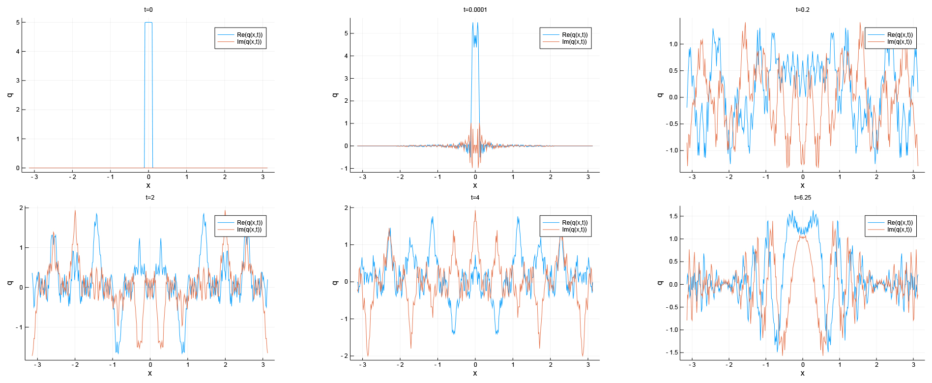
Figure 1. The solution at various times.
But when the solution is plotted at times rational multiples of \(2\pi\) (henceforth, rational times), a very different pattern emerges, as displayed in figure 2.
Apparently, this is a linear superposition of several copies of the initial datum, shifted regularly by a fraction of the period.
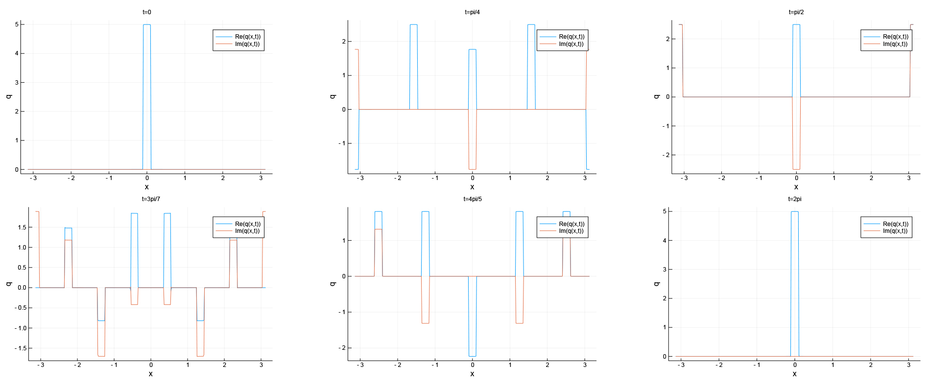
Figure 2. The solution at various times commensurate with \(\pi\).
If \(t=2\pi\), then \(e^{i(kx-k^2t)}=e^{i(kx-k^22\pi)}=e^{ikx}\) and the solution reduces to exactly the initial datum, so exact revivals of the initial datum and time periodicity of the solution are not wildly surprising, but revivals at other rational times \(t=2\pi\frac{p}{q}\), where \(\frac{p}{q}\) is a rational in reduced form, warrant further explanation.
Consider the Fourier series for the shifted initial datum
| |
\( q_0(x-r) = \frac{1}{2\pi} + \sum_{k\in{\mathbb Z}\setminus\{0\}}\frac{\sin(k\epsilon)e^{i(kx-kr)}}{k\epsilon2\pi}, \) |
|
in which we assume that \(q_0\) is itself a periodic function.
This formula is remarkably similar to the solution formula, except that the factor \(e^{-ik^22\pi p/q}\) in each term has been replaced by \(e^{-ikr}\).
Following the suggestion of the numerical experiments, we take a linear combination of \(q\) of these copies of the initial datum, each shifted by \(2\pi/q\) more than the last.
We find
| |
\( \sum_{j=0}^{q-1}A_jq_0\left(x-\frac{jp}{q}2\pi\right) = \sum_{j=0}^{q-1}\frac{A_j}{2\pi} + \sum_{k\in{\mathbb Z}\setminus\{0\}}\frac{\sin(k\epsilon)}{k\epsilon2\pi}e^{ikx}\sum_{j=0}^{q-1}A_je^{-ik\frac{jp}{q}2\pi}. \) |
|
For this to be another representation of \(q(x,t)\), it must hold that the \(A_j\) sum to 1 and, for all \(k\in{\mathbb Z}\setminus\{0\}\),
| |
\( e^{-ik^22\pi\frac{p}{q}} = \sum_{j=0}^{q-1}A_je^{-ik\frac{jp}{q}2\pi}. \) |
|
At first, this appears to be a grossly overspecified linear system, with only \(q\) degrees of freedom, but countably infinitely many equations.
However, representing \(k=uq+v\) for integer \(u\) and \(v\in\{0,1,\ldots,q-1\}\), we find
| |
\( e^{-ik^22\pi\frac{p}{q}} = e^{-2\pi ip\left(u^2q+2uv+\frac{v^2}{q}\right)} = e^{-iv^22\pi\frac{p}{q}}, \) |
|
and similarly for the linear combination on the right, so the system is equivalent to
| |
\( e^{-iv^22\pi\frac{p}{q}} = \sum_{j=0}^{q-1}A_je^{-iv\frac{jp}{q}2\pi}, \qquad v\in\{0,1,\ldots,q-1\}; \) |
|
note that the \(v=0\) case reduces to the \(A_j\) having unit sum.
This system is represented by a Vandermonde matrix whose rows are each generated by a different root of unity, so it is full rank.
Therefore, by solving the system, we may identify coefficients \(A_j\) for which
| |
\( q\left(x,\frac{2\pi p}{q}\right) = \sum_{j=0}^{q-1}A_jq_0\left(x-\frac{jp}{q}2\pi\right); \) |
(1) |
the solution at time \(2\pi p/q\) is a linear combination of \(q\) regularly spaced shifts of the initial datum.
The above calculation does not explain the smoothing at irrational times, but rational time discontinuities for discontinuous data, and Talbot's revivals at certain distances from the grating (times) are thereby explained.
Because Talbot worked with white light, he saw the superposition of solutions of the linear Schrödinger equation with dispersion relations scaled by a range of different positive constants corresponding to the frequencies of colors of light.
For each color, \(t\) must be scaled by this coefficient (and the period of the grating), leading to revivals at different distances for different colors.
Talbot did not see a more complex revival pattern for one colour at distances far from any distance with small \(q\) because at such distances there would always be another color for which the distance was closer to a smaller \(q\), producing a sharper revival for the latter color, hiding the more complex but less intense revival of the former.
Taking the limit as \(\epsilon\to0^+\), one obtains the fundamental solution of the initial boundary value problem, so it immediately follows that equation (1) is valid for any initial datum that is a test function for \(\delta\).
4. Smoothing of rough data at irrational times
Talbot's experiments, "communicated in the hope that they may prove interesting to the cultivators of optical science" were given some theoretical attention by Rayleigh and others in the physics community, but mathematicians paid little heed before 1992, when Oskolkov presented the first rigorous results.
In [15], periodic initial boundary value problems were studied, for linear partial differential equations with polynomial dispersion relations having integer coefficients, using the partial Fourier series of the sawtooth function, described as discrete Hilbert transforms, and collapsing to Gauss sums at rational times.
Oskolkov proved that at irrational times, the solution is continuous provided the initial datum is of bounded variation.
This irrational time smoothing is contrasted with Oskolkov's rational time result that discontinuities in the initial data produce discontinuities in the solution.
In 1996, Berry and Klein interpreted Talbot's experiment in geometric optics, studying solution curves along various lines [2]. They found the same Fourier series as arise in the zero potential linear Schrödinger equation, reducing to Gauss sums in formulae for the solution at rational times.
For constant \(x\), constant \(t\) (Talbot's first experiment), and certain \((x,t)\) diagonals (Talbot's oblique experiments), they found different fractal (Minkowski) dimensions of the solution curves.
Their results were proved rigorously in [10,16].
In [1], Berry extended the work of [2] to multiple dimensions, but only the separable case of rectangular periodicity appearing in Talbot's experiments.
Berry also conjectured that nonzero potential and nonlinear perturbations of the linear Schrödinger equation would preserve the fractal dimension results.
Erdoğan, Tzirakis, and their collaborators took up the challenge of proving the nonlinearization part of Berry's conjecture, and extending it to the class of integer polynomial dispersive equations studied by Oskolkov.
These works also provide an analytic explanation for the numerical studies of fractalization by Olver and collaborators, described below.
In 2013, Erdoğan and Tzirakis considered the cubic nonlinear Schrödinger equation on a periodic domain with initial data of bounded variation [9].
To address Berry's conjecture, they proved that the effect of the nonlinear perturbation is smoother than the purely linear evolution, a nonlinear smoothing result analagous to their result for the Korteweg-de Vries equation [8].
With this tool, they were able to quantify the irrational time fractalization in terms of bounds on the Minkowski dimension.
Because the equation is nonlinear, the rational time result is not characterized via revivals, but as lower regularity, at most countably many discontinuities, than at irrational times.
In 2015, togther with Chousionis, Erdoğan and Tzirakis obtained more Minkowski dimension fractalization results, this time for dispersive linear partial differential equations with monomial dispersion relation [5].
They also obtained similar results on the real and imaginary parts of the solution separately.
All these Minkowski dimension results give both upper and lower bounds on the Minkowski dimension, provided the initial datum is of bounded variation, but is irregular enough, quantified in a Sobolev sense.
Erdoğan and Shakan studied the nonlinear Schrödinger equation, the Korteweg-de Vries equation and their linearizations on \((x,t)\) diagonals [7].
They obtained Minkowski dimension bounds first for the linearizations, then nonlinearized using nonlinear smoothing results [9,8], tightening the Minkowski dimension bounds established in [5].
The introduction of [7] also provides an excellent and rather complete survey of irrational time smoothing and fractalization results.
The vortex filament equation models dynamics of a 1-dimensional vortex in a 3-dimensional homogenous incompressible inviscid fluid, and reduces to the cubic nonlinear Schrödinger equation under Hasimoto's transformation.
The initial datum for the vortex filament equation is the initial shape of the vortex filament, and polygonal initial data interested de la Hoz and Vega [6].
Hasimoto's transformation causes a reduction by 2 in Sobolev regularity of initial data, so the corresponding nonlinear Schrödinger problem has finite linear combinations of delta functions for its initial data.
Some numerical evidence suggesting fractalization at irrational times is presented by de la Hoz and Vega.
Chousionis, Erdoğan and Tzirakis were unable to prove the numerical observations of [6] as the nonlinear Schrödinger equation is illposed for distributional data, but they obtained a fractalization result on the vortex filament equation for smoother data.
5. Revivals at rational times
While preparing exercises for his textbook [12], Olver rediscovered the revival phenomenon for the linearized KdV equation, in which \(\omega(k)=k^3\).
Presenting this result with a third order version of the above argument [11], Olver also showed how to generalize the revivals argument to dispersive partial differential equations with dispersion relation any polynomial with integer coefficients (multiplied by a common real number).
He also gave a good survey of many of the works neglected here and concluded with some open problems.
Olver, Sheils and Smith explored revivals for the zero potential linear Schrödinger equation with more complicated pseudoperiodic boundary conditions [14].
Following numerical experiments, we were able to show that revivals do not require periodicity or even conservation of energy to occur, although the simple revival formula (1) is replaced with a more complicated version including also reflections of the initial datum.
For more general two point boundary conditions, other revival type phenomena are observed numerically, but not studied analytically.
Chen and Olver used numerical evidence to classify periodic dispersive wave equations with nonpolynomial dispersion relations, according to large wave number dynamics [3].
They identified some kind of revivals and fractalization for linearizations of Benjamin-Ono, Boussinesq and Benjamin-Bona-Mahoney, among others.
The rational time "revivals" are not exactly linear combinations of shifts of the initial data, but appear to be remarkably simple sums of something for small \(q\).
What that thing might be is not explored numerically or analytically.
Work in preparation by Olver, Pelloni and Smith begins to explore this question, providing analytic characterization of the rational time revivals for some linear dispersive equations with nonpolynomial dispersion relations.
Dispersive Lamb systems, in which the inhomogeneity is moved from the initial datum to an oscillating point mass, model transverse disturbances in a string or, depending upon the dispersion relation, another medium.
With periodic boundary conditions, the string is understood to be a loop.
In contrast to the results of [3], the numerical studies of Lamb systems by Olver and Sheils concluded that fractalization requires asymptotically sublinear growth of the dispersion relation [13].
There is no explicitly stated revivals result, but linearity means that revivals results similar to [3] would apply if an inhomogeneous initial condition were applied.
Erdogan and Shakan [7] provide some analytic discussion of the breakdown of revival phenomena for dispersion relations that are not integer coefficient polynomials, as observed in [3,13], albeit for the fractional Schrödinger equation which was not explicitly studied in either of those works.
Chen and Olver also studied weakly nonlinear systems numerically [3], and continued that work in [4].
In particular, they present numerical evidence for "revivals" and fractalization of integrable and nonintegrable nonlinear Schrödinger and Korteweg-de Vries equations.
Perhaps the strongest nonlinear revival result appears in the work of de la Hoz and Vega for the vortex filament equation.
They were able to establish that the rational time solution is polygonal if the initial datum is polygonal.
6. Some open problems
The following is by no means an exhaustive list, but offers a few questions the author considers interesting.
Some of these problems are intentionally left ill defined, suggesting ideas for further study, rather than specific conjectures.
- From [15], we understand that, as a sequence of rational time solutions approaches an irrational time limit, the jump discontinuities smooth out to give a limit function that is continuous. But precisely how that limit occurs, the possible heights of the jumps at rational times with large denominator is not fully understood.
- Precise fractal dimensions for solutions of nonlinear perturbations of dispersive partial differential equations have not been established, but the nonlinear smoothing results of Erdoğan and Tzirakis provide some good evidence for the nonlinearization part of Berry's conjecture.
- Fractalization and irrational time smoothing are reasonably clearly defined, even if the precise fractal dimension remains elusive in general and only bounded in many settings. In contrast, at rational times, there is a huge gap between the generally applicable "less smoothing" results of [15,9] and the proofs of genuine revivals demonstrated above for the periodic zero potential linear Schrödinger and presented in [11,14] other relatively simple circumstances. To fill this gap requires a good definition capturing the more general concept of revival that appears in the numerical studies of [3,14] and elsewhere.
- There is significant difficulty in extending results such as [14] to other equations, even with monomial dispersion relation. This arises from the fact that, except if the boundary conditions are periodic, the eigenvalues are not powers of integers. Similar problems occur in a general analytic treatment of the revivals observed numerically in [3]. Analytic results would certainly require the more general definiton of revival sought above, and it appears that a notion of convolution for generalized Fourier series, such as those arising from the Fokas transform method, would be valuable here.
- Berry conjectured that the perturbation of a linear dispersive partial differential equation by a smooth potential would preserve fractalization. This author's unpublished numerical studies suggest that revivals are also, in some sense, preserved by a smooth potential perturbation. But this has not been systematically studied.
Acknowledgement
The author thanks Peter Olver for useful conversations. The author would like to thank the Sydney Mathematics Research Institute for support and hospitality under the International Visitor Programme, and gratefully acknowledges support from Yale-NUS College workshop grant IG18-CW003.
References
[1] M. V. Berry, Quantum fractals in boxes, J. Phys. A: Math. Gen., 29 (1996), pp. 6617–6629.
[2] M. V. Berry and S. Klein, Integer fractional and fractal Talbot effects, J. Mod. Optics, 43 (1996), pp. 2139–2164.
[3] G. Chen and P. J. Olver, Dispersion of discontinuous periodic waves, Proc. R. Soc. Lond. Ser. A Math. Phys. Eng. Sci., 469 (2012), p. 20120407.
[4] G. Chen and P. J. Olver, Numerical simulation of nonlinear dispersive quantization, Discrete Cont. Dyn. Syst. A, 34 (2013), pp. 991–1008.
[5] V. Chousionis, M. B. Erdoğan, and N. Tzirakis, Fractal solutions of linear and nonlinear dispersive partial differential equations, Proc. London Math. Soc., 110 (2015), pp. 543–564.
[6] F. de la Hoz and L. Vega, Vortex filament equation for a regular polygon, Nonlinearity, 27 (2014), p. 3031.
[7] M. B. Erdoğan and G. Shakan, Fractal solutions of dispersive partial differential equations on the torus, Selecta Math., 25 (2019), p. 11.
[8] M. B. Erdoğan and N. Tzirakis, Global smoothing for the periodic KdV evolution, Int. Math. Res. Notices, 2013, pp. 4589–4614.
[9] M. B. Erdoğan and N. Tzirakis, The talbot effect for the cubic non-linear Schrödinger equation on the torus, Math. Res. Lett., 20 (2013), pp. 1081–1090.
[10] L. Kaptianski and I. Rodnianski, Does a quantum particle know the time?, in Emerging applications of number theory, D. Hejhal, J. Friedman, M. C. Gutzwiller, and A. M. Odlyzko, eds., vol. 109 of IMA Volumes in Mathematics and its Applications, Springer Verlag, New York, 1999, pp. 355–371.
[11] P. J. Olver, Dispersive Quantization, Amer. Math. Monthly, 117 (2010), pp. 599–610.
[12] P. J. Olver, Introduction to partial differential equations, Undergraduate texts in mathematics, Springer, 2014.
[13] P. J. Olver and N. E. Sheils, Dispersive lamb systems, J. Geom. Mech., 11 (2019), pp. 239–254.
[14] P. J. Olver, N. E. Sheils, and D. A. Smith, Revivals in the linear free space Schrödinger equation, Quart. Appl. Math., 78 (2020), pp. 161–192.
[15] K. I. Oskolkov, A class of I. M. Vinogradov's series and its applications in harmonic analysis, Springer, New York, 1992, pp. 353–402.
[16] I. Rodnianski, Fractal solutions of the schrodinger equation, in Nonlinear PDE’s, dynamics and continuum physics, J. Bona, K. Saxton, and R. Saxton, eds., vol. 255 of Contemp. Math., AMS, Rhode Island, 2000, pp. 181–187.
[17] H. F. Talbot, Facts related to optical science. No. IV, Philos. Mag., 9 (1836), pp. 401–407.